
I recently had to perform some analysis on a set of insurance companies in certain geography. After searching the net I found such list of companies operating in that continent. But the problem is,
- These companies are listed multiple times, one time for each of their geographical area of operation.
- I cannot count each company only once since there is geography specific operational data in that list.
- But at the same time, information pertaining to organization like total sales, strategy etc. are common to all the subsidiaries / separate entities of a company.
- There are too many companies to do the manual grouping of companies
I think this type of problems are fairly common in business analytics. So here is a relatively simple solution for getting unique list of companies without losing any information or writing macros. See the example for yourself.
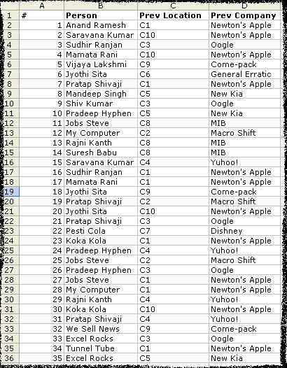
Lets take an example of employee data. You have fields like Person Name (sometimes unique), Previous employment, Previous workplace, Previous Salary. Now, if person Anand worked in more than one place earlier, there will be more than one rows with his name. But for details like DOB, SSN etc. there wont be multiple rows. So you need to know how many uniques rows are there in that huge list. Detailed Steps:
- Enter / copy the data

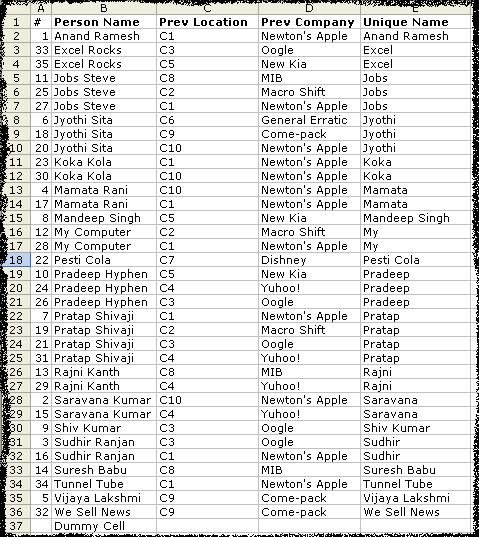
- Sort the list on person name

- In the column next to prev-company enter the following formula in E2
=IF(OR(LEFT(B2,SEARCH(" ",B2))=LEFT(B3,SEARCH(" ",B3)),LEFT(B2,SEARCH(" ",B2))=LEFT(B1,SEARCH(" ",B1))),LEFT(B2,SEARCH(" ",B2)),B2)
Copy – paste the formula in all the cells in the list for the column. You will see the followin result.

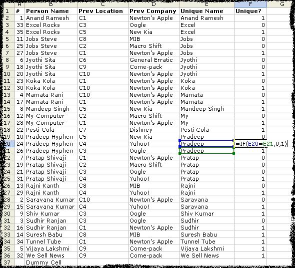
- Now create one more column next to Unique Name with heading Unique?. Paste the following formula in the F2. Apply the formula to all the cells in the list.
=IF(E2=E3,0,1)
Now, you would see the list like this.

- Now sellect the top row and apply “auto filters” [Data->Filter->Auto-Filter] And select 1 in the Unique? column. You will see all the unique names. You can copy paste this list in another sheet/work-book and work with it or assign corresponding codes to each of the unique items in this list.


To summerize:
1. Sort your list first.
2. Get the unique parts like first word / first number etc in another column. In my case I had to use first word.
3. Compare consecutive rows and mark the differences. Now you know how many unique items you have.
Comments / Any better ways of doing this are always welcome.


11 Responses to “Use Alt+Enter to get multiple lines in a cell [spreadcheats]”
@Chandoo:
One more useful trick.......
In a column you have no. of data in rows and need to copy in the next row from the previous row, no need to go for the previous rows but entering Alt + down arrow, you will get the list of data, (in asending order), entered in the previous rows...
This is another great tip. I use this all the time to make sense of some *very* long formulas. As soon as the formula is debugged I remove the break.
Great tip Chandoo!
I use this feature often and it has even gotten the, "how did you do that" response.
Thanks!
@Ketan: Alt+down arrow is an awesome tip. I never knew it and now I am using it everyday.
@Jorge, Tony: Agree... 🙂
[...] Day 1: Insert Line Breaks in a Cell [...]
how can we merge a two sheet.
excellent idea. Chandoo you are genious
Hi chandoo,
I have used ctrl+enter to break the cell. But I did not get the result.
Please tell me how can i break the cell in multiple lines.
Hi, Ranveer,
Its not Ctrl+enter to break the cell, use Alt+Enter to make it happen.
hi Chandoo....
how we can use Alt+Enter in multiple rows at the same time please reply hurry i have lot of work and have no time and i m stuck in this. 🙁
Alt+J worked once 🙁
So I found another more reliable way:
=SUBSTITUTE(A2,CHAR(13),"")
Where A2 is the cell that contains the line breaks which the code for it is CHAR(13). It will replace it with whatever inside the ""