
Here is tricky scenario, faced by Basil, our forum member,
I want to have Excel display a wing ding check mark when a user types “y” in a cell. I have been trying to do a substitute formula but putting the symbol in an unused portion of the spreadsheet and calling it to the selected cell but I can’t get it to work. Any thoughts? [more]
There are 2 simple solutions I can think of (other than the solution proposed by Axim5)
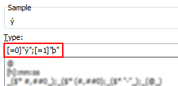
1. Using custom cell formatting
This approach is more robust, but a compromise. Instead of “y” and “n”, user should type “1” and “0”. Then we can use custom number formatting to conditionally display the tick mark symbols.
PS: you need to change the font to “wingdings”. 🙂
See this:

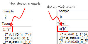
2. Using conditional formatting
[This method works only in Excel 2007 and above]
Starting with excel 2007, you can use conditional formatting to set cell format codes as well. This means, when the cell value is Y, we can conditional format the cell to show tick mark symbol. All you have to do is define a new rule, and then go to “number” tab and set the format code you want.
For eg. a code like this will give an output shown to the right.
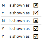
There you go Basil. Go check all you want.
More resources on cell formatting and conditional formatting:
- Excel Conditional Formatting – 5 tips and tutorials
- Number Formatting in Excel – Tips
- Hiding a cell’s contents using conditional cell formatting
- Number format codes + Chart Labels = Pure fun
What is your favorite number formatting trick?
Share with us using comments.


26 Responses to “FIFA Worldcup Excel Spreadsheets [Roundup]”
Nice roundup! Do you know of any one-page spreadsheets which will be updated by an administrator after each game? Would be nice to be able to print out the latest results whenever I feel like checking them as I probably won't be following closely every day.
I actually haven't tried any of the above ones yet, but I thought I'd mention this one that I found which makes a nice one-page form you can fill in dynamically. http://exceltemplate.net/sports/world-cup-2010-schedule-and-scoresheet/
I would like to recommend you these one: http://www.anotagol.com/
You can choose your interface language (english, spanish, italian, portuguese, german or french) and your country for the timezone of match. I like it very much.
An awesome online world cup calendar in flash.
http://www.marca.com/deporte/futbol/mundial/sudafrica-2010/calendario-english.html
Got one more tracker in excel (one page)
http://cid-b09e57e6e960505c.office.live.com/browse.aspx/.Public
[...] Passend zu gerade laufenden Fußball-WM gibt es auf Chandoo.org alles wissenswerte über Excel-Anwendungen für den Fußball-Fan. [...]
Great!!!
I strongly recommend this :
http://www.en.excel-soccer-2010.de/downloads
Chandoo how you found this ...
@Rohit.. really beautiful file. I missed it during my research. Now, I recommend it. 🙂
Hi Chandoo - thanks for the recommandation 🙂 - Regards
[...] Excel, then print it on the other side of your Match Schedule from step 2 above. There are several other Excel spreadsheet templates you can download, but this is probably the only one-page version you can find; plus, it [...]
Does anybody know how to re-create this(?): http://www.marca.com/deporte/futbol/mundial/sudafrica-2010/calendario-english.html
...or do you know where a template can be found? I am DYING to have something like this on my site. When I found it, I had been looking for the longest time for a circular calendar. I found a couple that weren't adequate. Then I stumbled upon this one and my eyes nearly popped out of my head. If anyone can lead me in the right direction, I would be eternally grateful!
Thanks in advance!
Robert
@Robert...
Doing something like that is a lot of work. You can probably get it done with some hired help from a flash developer.
@Robert, the World Cup flash in the Spanish Marca newspaper is impresive, but not much as my own animated spreadsheet with the Goals of 2010 World Cup South Africa in Excel that I just published into my blog:
http://pedrowave.blogspot.com/2010/06/goals-of-2010-world-cup-south-africa-in.html
Download from here:
http://cid-6b219f16da7128e3.office.live.com/view.aspx/.Public/Goals%20South%20Africa%20Animated.xlsx
And start to enter the goals of the rest of matches.
Has anyone seen, or made, a Spreadsheet where you can record the scorers and see a 'top scorers' chart. Would be a nice enhancement
@Neil... checkout this one http://www.inflexionary.com/sports/world-cup-2010-excel
it uses macros to fetch scores from web (and provides very comprehensive analysis too)
@All.. Thanks for the comments. I have updated the post with few more links now.
Hi,
Check this dashboards too:
http://dashboards.org/world-cup-dashboards-and-visualizations/
😉
[...] Here is a collection of FIFA World Cup Spreadsheets if you are more in to that sort of thing. | [...]
[...] Cup fever is here!In FIFA Worldcup Excel Spreadsheets Roundup, Chandoo has some links to useful World Cup tracking workbooks. Only one of them (the first one) [...]
[...] World Cup fever is here!In FIFA Worldcup Excel Spreadsheets Roundup, Chandoo has some links to useful World Cup tracking workbooks. Only one of them (the first one) [...]
Hey, you missed ours! It has everything you need and more, but not a whole pile of silly extras (National Anthems, etc). I'll be making another one for the 2014 world cup. We had over 4000 hits on it!
@Michael Harwood.
Where is it then? You should have posted a link
Sie sollten an einem Wettbewerb teil zu nehmen für einen der besten Blogs im Web. Ich werde empfehlen Sie diese Seite!
Google translation: You should take part in a contest for one of the best blogs on the web. I will recommend this site!
[...] and welcome to the forum, Maybe these similar spreadsheets might give you a few initial ideas: FIFA Worldcup Excel Spreadsheets [Roundup] | Chandoo.org - Learn Microsoft Excel Online If you have specific areas / formulae / layout choices for parts of your spreadsheet that you are [...]
Calling all football fans around the globe! The biggest football festival will kick off on the 12th June 2014 and everyone is placing their bets of who will have the honour of lifting the golden trophy.
Use our free interactive Excel templatel to predict the World cup finalists ! No macros !
http://www.spreadsheet1.com/world-cup-2014-free-excel-prediction-template.html
I also made a Worldcup-tracker, with MS Access, which can also generate reports in Excel
e.g. a match-schedule with locations on y-axis and dates on x-axis, see:
http://worktimesheet2014.blogspot.com.es/2014/05/excel-with-match-schedule-for-2014-fifa.html
and:
http://worktimesheet2014.blogspot.com.es/2014/05/match-access-app-to-track-world-cup.html
where can i find raw data in excel file format of fifa world cups (1930-2014)
@Vivek
Have a read of: http://chandoo.org/forum/threads/goal-of-world-cup.17637/
The location is mentioned in Somendra's comments
Free XLSX Prediction Spreadsheet for World Cup 2018 Russia!
https://www.spreadsheet1.com/fifa-world-cup-2018-russia-free-prediction-templates-for-excel.html