Even Faster Way to Compare 2 Lists in Excel [Quick Tip]

Share

Facebook
Twitter
LinkedIn

Last week we discussed a fun and easy way to compare two lists of data in excel using conditional formatting. In that post, Artem commented,

The quickest way to find all about two lists is to select them both and them click on Conditional Formatting -> Highlight cells rules -> Duplicate Values (Excel 2007). The result is that it highlights in both lists the values that ARE the same. Then in one list non-highlighted are values that are not present in the second list, and opposite for the second list. I think it is sell “geeky”, but it gets job done very very quickly when you don’t want to mess around.

Artem must be an Excel Yoda. I somehow missed this beautiful and dead-simple way to compare lists in Excel. So here, I am documenting that technique so we all remember it and use it.

A Ridiculously easy and fun way to compare 2 lists
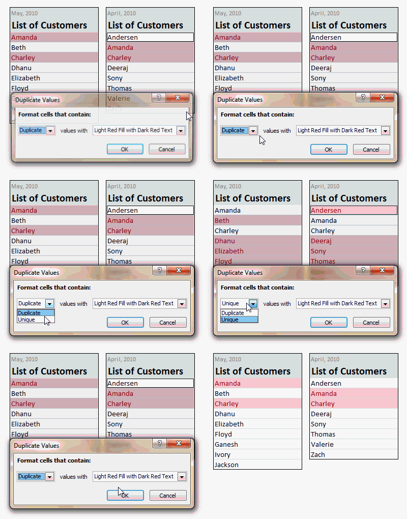
Compare 2 lists of Data in Excel - Conditional Formatting Tip[works only Excel 2007+, use the above technique if you are on excel 2003 or earlier]

  1. Select cells in both lists (select first list, then hold CTRL key and then select the second)
  2. Go to Conditional Formatting > Highlight Cells Rules > Duplicate Values
  3. Press ok.
  4. There is nothing do here. Go out and play!

See the screencast aside to see how this works (click here for a detailed demo).

Hats off to Artem for sharing this beautiful tip with us. Thank you 🙂

Spare a minute to become superawesome at work – Read a Quick Tip.

Facebook
Twitter
LinkedIn

Share this tip with your colleagues

Excel and Power BI tips - Chandoo.org Newsletter

Get FREE Excel + Power BI Tips

Simple, fun and useful emails, once per week.

Learn & be awesome.

Welcome to Chandoo.org

Thank you so much for visiting. My aim is to make you awesome in Excel & Power BI. I do this by sharing videos, tips, examples and downloads on this website. There are more than 1,000 pages with all things Excel, Power BI, Dashboards & VBA here. Go ahead and spend few minutes to be AWESOME.

Read my storyFREE Excel tips book

Overall I learned a lot and I thought you did a great job of explaining how to do things. This will definitely elevate my reporting in the future.
Rebekah S
Reporting Analyst
Excel formula list - 100+ examples and howto guide for you

From simple to complex, there is a formula for every occasion. Check out the list now.

Calendars, invoices, trackers and much more. All free, fun and fantastic.

Advanced Pivot Table tricks

Power Query, Data model, DAX, Filters, Slicers, Conditional formats and beautiful charts. It's all here.

Still on fence about Power BI? In this getting started guide, learn what is Power BI, how to get it and how to create your first report from scratch.

22 Responses to “Formula Forensic No 019. Converting uneven Text Strings to Time”

  1. Joe Carsto says:

    Why not let the TIME function take care of the math:
    =TIME(LEFT(TEXT(A1,"000000"),2),MID(TEXT(A1,"000000"),3,2),RIGHT(TEXT(A1,"000000"),2))

    • Ben Niebuhr says:

      I was going to point out the same thing, except to note that useing the time function and doing the divide method are not interchangeable.

      I have spent hours investigating a spreadsheet working with a couple of years worth of hourly data, and found that the reason things weren't working is because the rounding on the divide method is only close to the correct time values. In order to have it work for comparisons, (like sub-totaling by time value, or pivoting) you MUST use the TIME function.

      Great use of the TEXT function, Hui. I will be using this concept for sure.

  2. Elias says:

    Why not just.

    =TEXT(A1,"00\:00\:00")*1

    Regards

    • Joe Carsto says:

      Elegant!

    • Manick says:

      Hi Elias,

      I tried to use your formula. But, it doesn't seem to work for me. I am getting an error message "The formula you typed contains an error". It seems I have the problem in using \: in the format. How can I overcome this?

      Thanks

      • Greg G says:

        Manick, it isn't the /: that causes the problem. If you copy/paste it, you're getting “'s instead of the actual quotation marks that Excel uses. Change the quotation marks by deleting from the pasted formula and retype them.

      • modeste says:

        Hi Manick...
        use this alternate formula :
        =1*TEXT(A1,"00"":""00"":""00")

        note twice double quote each side of :

  3. Elias says:

    @Manick,

    Did you copy the formula and pasted in Excel or did you typed? Also, do you use , or ; as separator of arguments?

    Regards

    • Joe Carsto says:

      @Elias: I had no problem using your formula, in fact, I have used your method to convert a number such as 20120419 to an Excel date using =TEXT(A1,"0000\/00\/00")*1. Thanks for posting.

      • Elias says:

        @Joe: For date convertion you can use this as well.

        =TEXT(A1,"00-00-00")*1

        Regards

        • Joe Carsto says:

          Sweet! It appears this also works with =TEXT(A1,"0-00-00")*1. I come from the old days when you counted every byte. I also like to try an make formulas as small as possible for the fun of it 🙂

  4. Haseen says:

    Elias's suggestion is the simplest, but here is yet another way with TIME and MOD functions...

    =TIME(MOD(A2/10000,100),MOD(A2/100,100),MOD(A2,100))

  5. Since the seconds appear to always be 0, why not simply the input to minutes and above and save yourself the trouble of typing those zeroes...

    0 => 0:00
    1 => 1:00
    10 => 10:00
    100 => 1:00:00
    etc.

    Then just use this formula...

    =TEXT(A1,"0\:00\:")*1

    • Elias says:

      @ Rick, the numbers to convert are no typed, they are imported. Then your formula will return the wrong result.

      Regards.

  6. Hmm! My formula lost some backslash-zero combinations (two of them to be exact). The formula was supposed to be this...

    =TEXT(A1,"0\:00\:\zero\zero")*1

    where the words "zero" should actually be the number 0. Another way to write the formula is this...

    =TEXT(A1,"0\:00\:""00""")*1

  7. Rajagopal says:

    Hi Master,
    While writing the formulae you have considered only upto "seconds factor" . I think you should take the centi-seconds factor also to achieve best results. Please look into it and rectify the problem...?

    For Example.
    In horse racing timings are noted in minute, seconds and centi-seconds, like if a horse finished in 70 seconds over a scurry of 1200 metres, is noted as 1.10 min. Nowadays it is noted in centi-seconds everywhere, like 70.00 if you want to convert it to centi seconds (should multiply by 100) = 7000 centi seconds. If you put this figure into your formula as a general number (7000) it will return as 1:10:00. As per your formula, it should be taken as 1 hour 10 seconds 0 minutes. However for a racing enthusiast like me it can be taken as 1 minute 10 seconds also.

    Just look what happens if we race goers use this figure as 7000 centi seconds in your formulae, it will correctly show as 1 minute 10 seconds(?) Suppose a horse finishing over a 1200m in 70.60 seconds or in racing terms written as 1.10.60 mins, where 1 minute 10 seconds, & 60 centi-seconds can be counted as 7060, if you put this figure in the formula it will return as 1 minute 11 seconds, that is correct.

    My point is if you can incorporate Centi Seconds in the formulae, it would be of great help to us also.

    Thanks and regards.
    Rajagopal (Mumbai)

  8. Vishy says:

    Awesome techniques !

    I tried with 235960 just to see if it will fail but this is great.

  9. CMC says:

    Although a little longer, this too work:

    =CHOOSE(LEN(A2);A2/(24*3600);A2/(24*3600);LEFT(A2;1)/(24*60) + RIGHT(A2;2)/(24*3600);LEFT(A2;2)/(24*60) + RIGHT(A2;2)/(24*3600);LEFT(A2;1)/24 + MID(A2;2;2)/(24*60) + RIGHT(A2;2)/(24*3600);LEFT(A2;2)/24 + MID(A2;3;2)/(24*60) + RIGHT(A2;2)/(24*3600))

  10. Converting uneven Text Strings to Time I have imported some data that comes in as a number that I need to convert to h:mm.

  11. Sudhir Gawade says:

    Just come across this while googling

    find interesting challenge and come up with this 

    =TEXT(TEXT(SUBSTITUTE(A1,RIGHT(A1,1),""),"000000"),"00\:00\:00")

  12. Renee Keel says:

    I need to convert a string of numbers representing average minutes, to reflect correct time values. For example, the numbers below currently represent 5.79 minutes, 15.82 minutes, etc.

    I need to convert these values to their correct corresponding value within time parameters. So 5.79 would be something close to 5 minutes and 45 seconds.

    5.79
    15.82
    3.92
    12.40
    6.70
    3.62

    I know there has to be a way to compute this in Excel, it can do anything, I believe!

    Thank you for any and all assistance~

    • Chandoo says:

      @Renee... You can use a formula like this. Assuming A1 has the minutes.seconds,

      =INT(A1) + MOD(A1, 1)*0.6

      If you want to see it in 5 minutes 45 seconds format, use

      =INT(A1) & " mins " & ROUND(MOD(A1, 1)*0.6,2) & " secs"

Leave a Reply