Since Financial Modeling School 2nd batch is opening next week, things have been a bit crazy at chandoo.org HQ.
So we will start the week with an ultra quick tip. It always surprises me that not many people know this. So here it goes,
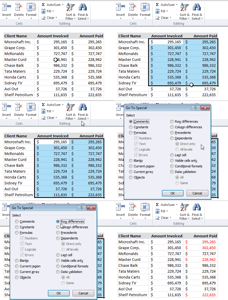
Lets say you have some data in 2 columns and you want to compare row by row to spot the differences. Of course you can write a formula or apply conditional formatting. But there is a quick and dirty solution that works just as fine.
- Select both columns with data
- Press F5 and select special (alternatively, from home ribbon, click on Find & Select and then choose Goto Special)
- Now, click on “row differences” and press OK.
- Excel instantly highlights all the cells in 2nd column that do not match with first column.
- Just change their color or something so you know where to focus your attention.
- Done!
See this demo to follow the steps:
Want more? Here is more:
- A ridiculously fast way to highlight mismatches in data using Conditional formatting
- Learn more quick tips and become an Excel rock-star.


13 Responses to “Convert fractional Excel time to hours & minutes [Quick tip]”
Hi Purna..
Again a great tip.. Its a great way to convert Fractional Time..
By the way.. Excel has two great and rarely used formula..
=DOLLARFR(7.8,60) and =DOLLARDE(7.48,60)
basically US Account person uses those to convert some currency denomination.. and we can use it to convert Year(i.e 3.11 Year = 3 year 11 month) and Week(6.5 week = 6 week 5 days), in the same manner...
This doesn't work for me. When applying the custom format of [h]:mm to 7.8 I get 187:12
Any ideas why?
@Jason
7.8 in Excel talk means 7.8 days
=7.8*24
=187.2 Hrs
=187 Hrs 12 Mins
If you follow Chandoo's instructions you will see that he divides the 7.8 by 24 to get it to a fraction of a day
Simple, assuming the fractional time is in cell A1,
Use below steps to convert it to hours & minutes:
1. In the target cell, write =A1/24
2. Select the target cell and press CTRL+1 to format it (you can also right click and select format cells)
3. Select Custom from “Number” tab and enter the code [h]:mm
4. Done!
Hi, sorry to point this out but Column C Header is misspelt 'Hours Palyed'
good one
So how do I go the other way and get hours and minutes to fractional time?
If you have 7.5 in cell A1,
- Use int(A1) to get the hours.
- Use mod(A1,1)*60 to get minutes.
If you have 7:30 (formatted as time) in A1
- Use hours(a1) to get hours
- Use minutes(a1) to get minutes.
I had the same issue. You can solve it by changing the format as described above:
Right click cell > Format Cells > (In Number tab) > Custom > Then enter the code [h]:mm
([hh]:mm and [hhh]:mm are nice too if you want to show leading zeros)
Thanks guys, these are the tips I'm looking for.
...dividing the number of minutes elapsed by the percent change is my task - "int" is the key this time
It doesnt work for greater than 24 hours
It returns 1:30 for 25.5 hours. It should have returned 25:30
Ideally I would right function as
=QUOTIENT(A1,1)&":"&MOD(A1,1)*60
Sorry, replied to wrong comment....
----
I had the same issue. You can solve it by changing the format as described above:
Right click cell > Format Cells > (In Number tab) > Custom > Then enter the code [h]:mm
([hh]:mm and [hhh]:mm are nice too if you want to show leading zeros)
Clever use of MOD here to extract the decimal part of a number. Divide a number containing a decimal by 1 and return the remainder. Humm. Very clever.
Thanks very much, extremely useful !