
Here is a charming little problem to kick start your day.
Lets say you run a cute little bakery around the corner. Since you want your prices to look charming, you have a policy to round them down or up based on below rule.
If the price ends with 0, 1 or 2 cents, round it down to 9 cents.
If the price ends with 3, 4 or 5 cents, round it up to 5 cents.
If the price ends with 6, 7, 8 or 9 cents, round it up to 9 cents.
For example,
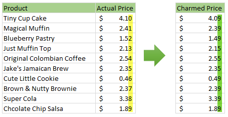
So how do you round to nearest charmed price? You could do it manually. But you would rather bake a few more of those Tiny Cup Cakes than waste time rounding the prices. So you want an automatic way to round prices. This is where Excel helps.
Formula for rounding to charmed price
There are many ways to write a formula for this.
The first and most obvious method is to use IF formula
Assuming regular price is in cell C4, The formula for charmed price would look like this:
=ROUNDDOWN(C4,1) + IF(MOD(C4,0.1)<=0.02,-0.01, IF(MOD(C4,0.1)<=0.05,0.05,0.09))
Go ahead and take a hard look at it.
The first that strikes us when you read it would be,
‘Gee, Thats one long formula. I need a coffee.’
How it works:
- First we round down the price (in C4) to 10 cents with ROUNDDOWN(C4,1)
- Then we add or subtract few cents to get the charmed price with IF formula.
- IF the cents are less than or equal to 0.02, we subtract 1 cent
- IF the cents are between 3 & 5, we add 5 cents.
- Else, we add 9 cents.
So for example, if the actual price is $2.37, the formula gives $2.39 thru below process.
- Price rounded down to 10 cents will give $2.30
- MOD(2.37,0.1) gives 0.07
- This is falls in to the else portion of 2nd IF formula
- IF(MOD(2.37,0.1)<=0.02,-0.01, IF(MOD(2.37,0.1)<=0.05,0.05,0.09))
- So we add 9 cents to the rounded down price.
- Hence the charmed price is $2.39
[Related: Introduction to IF formula]
An improvement – CHOOSE formula
If the IF formula is too long & difficult to write, we can choose CHOOSE formula.
It goes like this:
=C4 + CHOOSE(MOD(INT(C4*100),10)+1,-0.01,-0.02,-0.03,0.02,0.01,0,0.03,0.02,0.01,0)
This formula takes the price in C4 & adds or subtracts necessary cents to it to get the charmed price.
Examining it with $2.37 gives,
=2.37 + CHOOSE(MOD(INT(C4*100),10)+1,-0.01,-0.02,-0.03,0.02,0.01,0,0.03,0.02,0.01,0)
=2.37 + CHOOSE(8, -0.01,-0.02,-0.03,0.02,0.01,0,0.03,0.02,0.01,0)=2.37 + 0.02
=2.39
[Related: Introduction to CHOOSE formula]
VLOOKUP & A mapping table
We can simplify our CHOOSE formula with a mapping table.
Lets say, somewhere in the workbook, we have set up a mapping table like this:

Then, we can use VLOOKUP formula to calculate charmed price:
=C4+VLOOKUP(MOD(INT(C4*100),10), mapping.table, 2 ,FALSE)
This formula is similar to CHOOSE formula.
How it works?
Assuming actual price is $2.37,
=2.37 + VLOOKUP(MOD(INT(C4*100),10), mapping.table, 2 ,FALSE)
=2.37 + 0.02 = 2.39
[Related: Introduction to VLOOKUP formula]
VLOOKUP & A smaller mapping table
Using a combination of rounded down price & approximate lookup feature of VLOOKUP, we can come up with a smaller formula.
This requires a new mapping table like this:

Our formula now looks like this:
=ROUNDDOWN(C4,1) + VLOOKUP(MOD(INT(C4*100),10),new.mapping,2)
How it works?
=ROUNDDOWN(2.37,1) + VLOOKUP(MOD(INT(2.37*100),10),new.mapping,2)
=2.3 + VLOOKUP(MOD(237,10),new.mapping,2)
=2.3 + VLOOKUP(7,new.mapping,2)
=2.3 + 0.09
=2.39
Download Example Workbook
Click here to download charmed price example workbook. Examine it to understand various formulas discussed in this article.
Challenge for you – write another formula for charmed prices
Here is a challenge for you. Assuming the price is in C4, can you come up with another way to calculate charmed price? Please share your formulas in the comments section.
Go ahead and charm us.
Want to charm your boss? Learn these as well
Excel spreadsheets are like transmogrification cloaks. If you put on the right ones, you will instantly become incredibly charming. So learn how to weave powerful spreadsheets and charm everyone around you. Start with these:
- 18.2 tips to rounding numbers in Excel
- Calculating new prices after % hike
- IF formula challenge for you


14 Responses
The first IF statement isn’t working for me where the second decimal place is 0 – for me it is turning 4.10 into 4.19
My alternative:
=(IF(AND(MOD(INT(C4*100),10)>=3,MOD(INT(C4*100),10)<=5),5,9)+TRUNC(C4*10)*10+IF(MOD(INT(C4*100),10)<=2,-10))/100
Hi,
Wouldn´t be possible also to use a boolean logic formula. Built similar to the if but just adding the data. Probably it would be the most efficient one.
As a programmer, I think you are over-complicating the solution. It is a simple if statement and the rounddown. This formula works, it is fairly simple and other than Excel giving the wrong answer for mod(2.73,.1) = .2999999999998. It works:
=ROUNDDOWN(H1,1) + IF(AND(MOD(H1,0.1)-0.03>=0,MOD(H1,0.1)-0.03<=0.02),0.05,0.09)
@Jay.. thanks for the comments.
Excel has floating point error which can cause weird behavior when dealing with fractional arithmetic.
NOT an array formula:
=IF(OR({3,4,5}=MOD(C4*100,10)),ROUNDUP(C4,1)-0.05,ROUND(C4,1)-0.01)
Two more to ponder.
1st one:
=ROUND(C4,1)-0.01+CHOOSE(MOD(C4*100,10),,,6,6,-4,,,,)/100
2nd one:
{=ROUND(C4,1)-0.01+SUM(({3,4,5}=MOD(C4*100,10))*{6,6,-4}/100)}
A different approach: assuming in A1:B10 we have a helping table like this:
0 -0.01
1 -0.02
2 -0.03
3 0.02
4 0.01
5 0
6 0.03
7 0.02
8 0.01
9 0
and our prices start in cell D1 the shortest formula I found is:
=VLOOKUP(RIGHT(D1*100,1)*1,$A$1:$B$10,2,0)+D1
Cheers.
If the numbers have more decimals that aren´t shown because of format in the list given by chandoo your method would not work 🙁
I assume that given example is actually a price and those tend to not go further than 2 decimals (in $/cent example) – at least those I’ve seen so far 🙂
If I knew these aren’t actual prices (for example some calculated values) I would just simply round them – problem solved 🙂
I’d like to buy 10,000 Micro sampler cakes at the actual price of $0.02 each, please. Coooooeee, looks like you owe me $100! Thanks!
Jaja. True 🙂
IF(OR(RIGHT(A1;1)=”3″;RIGHT(A1;1)=”4″;RIGHT(A1;1)=”5″);MROUND(A1;0.05);ROUND(A1;1)-0.01)
Hi Guys,
I saw smart answers for this homework and hope to get to this level soon. Though i’m new here I give bellow a solution that is still long but works:
C4+IF(VALUE(RIGHT(100*C4,1))<=2,-(RIGHT(100*C4,1)+1)/100,IF(VALUE(RIGHT(100*C4,1))<=5,+(5-(RIGHT(100*C4,1)))/100,+(9-(RIGHT(100*C4,1)))/100))
Regards,