
 This post is part of our chartbusters series.
Ever since I was a child, I was fascinated by Paris (and Eiffel Tower). So much so that I even took french lessons during my post graduation in the hopes of one day traveling to the romantic land.
Recently, I had opportunity to visit Paris, albeit for just a few hours (I had a 12 hour lay-over in Paris between flights). I went to see the Eiffel Tower and it looked just as beautiful and majestic as it did in my imaginations.
But this is not a travel blog, it is a charting and excel community. So I have something for you as well.
During my visit to Eiffel tower, I took the stairs to 2nd floor and along the way they have a handful of visualizations explaining the tower. I found them quite interesting and well made. Here, I have listed down 4 simple, yet very effective visualization lessons for all of us.
Lesson 1: Compare with known things in your charts
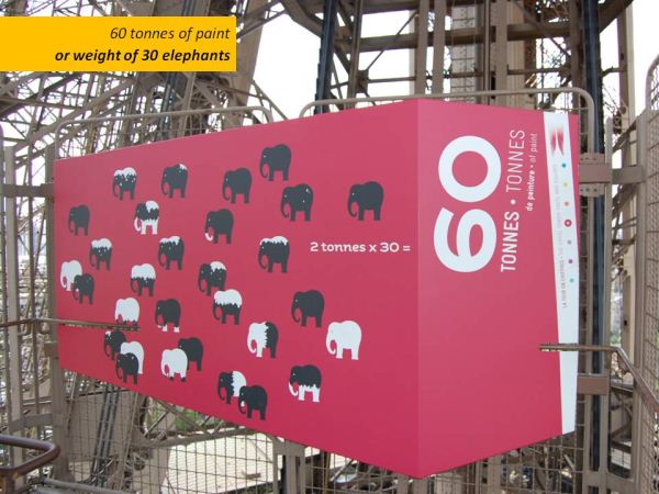
Eiffel tower is a huge tourist attraction with distinguished history. But you have to tell about it to scores of visitors everyday in easy to understand manner. Comparison is a very effective technique. It raises the curiosity and connects well with audience.
For eg. see how they have explained the fact that “Eiffel tower used 60 tonnes of paint”.
Lesson 2: Get creative, don’t always fallback on bar / pie charts
We all know that bar charts are very effective. But too many bars would make the charts look bland. Experimentation could lead to some creative solutions to bar (or pie) fatigue. [Related: 5 ways to dress up your charts]
For eg. see how they have compared the height of Eiffel tower with other familiar landmarks (it is still a bar chart, but creatively implemented)

Lesson 3: Sometimes just numbers will do
While charts add a lot of value (and provide insight), sometimes you want to limit yourself to just numbers.
For eg. they have shown the number 336 in large font along with an illustration of flood-lights to tell us that 336 floodlights light up the tower in the night.

Lesson 4: Focus on the the tower, not on charts
This, probably is the most important lesson of all. We are all here to build our own Eiffel tower and show it off to others. So it is important to focus on the tower, the charts are secondary.

I have made a small presentation with various visualizations showcased on the Eiffel Tower, each one teaches a valuable lesson on charting and story-telling. Take a look at it below:
if you are not able to view it in feed reader / e-mail, click here
Other charting lessons:


7 Responses
Very nice, Chandoo. Thanks for sharing this. I’ve heard plenty about the Eiffel Tower, visualization lessons from it is a first. I find #3 of special importance: many times we focus our energies on chart embellishments than thinking if the chart is even required.
PS: Now you’ve made me want to visit France too!
Excellent post Chandoo!
The guys who have created this visualization really understand their target audience well. A normal human being cannot grasp more than a few numbers. Had they used numbers or bars then after seeing so many of them you would remember nothing and understanding nothing.
But the way they have made ‘sense’ of large numbers and statistics is commendable.
I actually don’t care for the second one, it looks like a good idea ruined by poor presentation. The comparison between the landmarks is plenty interesting by itself, but the random placement of labels and the messy stacking just make the chart look busy without adding any value.
And as long as I’m nitpicking, the visualization seems to be drawing the eye away from the Eiffel Tower when it should arguably be the focal point. They should have sorted the stacks of landmarks from smallest to largest so that the Eiffel Tower was right next to the 324, which seems to be the visual center of the piece.
@Shuchi… Thank you. That is right, it is important to treat numbers as numbers in some cases. The temptation to make charts is way too much with such easily accessible tools and methods.
@Vivek: We can find such great visualizations all around us in zoos, highways, exhibitions and public attractions. The need for making simple and very effective graphs raises exponentially with increase in number of people seeing them.
@David: Thanks for sharing such a good point. I have a different view on it. Had they neatly stacked the buildings, it would have certainly looked bland and tasteless (atleast after climbing 300 stairs on a hot day). Since most of the visitors are students and kids (and people are usually in a very good mood after reaching the tower) it makes all the more sense to mis-align things to make it look peppy and fun.
Chandoo,
No doubt they spent very long hours to read your excellent Blog, as I do.
Many thanks for your web site.
One of your most regular french reader.
@Francois: That is so lovely. Thank you 🙂