Analyzing Search Keywords using Excel : Array Formulas in Real Life

Share

Facebook
Twitter
LinkedIn

Jarad asks me in an email “how word frequency can be generated from a range of cells using excel formulas?” This got me thinking and lead to this post, where we learn how to calculate word frequency using array formulas and use it to analyze a bunch of search keywords.

Array formulas are one of the powerful and often underutilized features of excel. They are often difficult to understand and use. But once you develop the ability write array formulas suddenly you see new possibilities.

If you are new to array formulas, read our excel array formulas tutorial

Step 1. Get your data

You must be so bored to see the same step no matter what we do. But getting the right data solves half the problems. Let us assume, our fictitious website has the following search keywords (well, really key phrases)
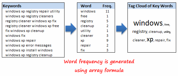
As a smart reader, you can already guess that in real life you will have not 10, but hundreds of key phrases that you would like to analyze. But the ideas you will be learning today should work in the same way.

Step 2. Calculate Word Frequencies using Array Formulas

First we must define the list of words for which frequency should be calculated. I just chose 9 arbitrary words. You can see them in the middle table.

Now we use array formula to calculate word frequency.

First the formula:

Assuming the keywords table (on the left) is in the range B4:B13 and the keyword for which you want to calculate the frequency is in D4, the array formula looks like,

=(SUM(LEN($B$4:$B$13))-SUM(LEN(SUBSTITUTE($B$4:$B$13,D4,""))))/LEN(D4)

Now the explanation

The frequency of the word in D4 (in this case it is “windows”) is calculated by,

  • finding the length of the entire text in the range b4:b13
  • finding the length of the entire text in the range b4:b13 after removing all occurrences of the word “windows”
  • Then, frequency is the gap between above 2 divided by the length of the word “windows”

Now look at the above formula.

SUM(LEN($B4:$B13)) is doing in the first part

SUM(LEN(SUBSTITUTE($B$4:$B$13,D4,""))) is doing the second part

/LEN(D4) is doing the last part.

Step 3. Finally Prepare a Tag Cloud from Keyword Frequencies

This is the simplest part of all, provided you have the tag cloud chart macro installed. When you have loads of keywords, tag cloud can help you visualize the important keywords.

What next?

You can take this basic model and extend it to include parameters like number of searches each key phrase has, how long the users stay on the site etc. to enhance the way tag cloud is generated and colored.

Also read some of the related text processing tricks using excel:

Sorting text using Excel Formulas

Find if a word is repeated in a cell

Cleanup incorrectly formatted phone numbers

Fuzzy text search using excel

Share with us how you use array formulas, your favorite tricks.

Facebook
Twitter
LinkedIn

Share this tip with your colleagues

Excel and Power BI tips - Chandoo.org Newsletter

Get FREE Excel + Power BI Tips

Simple, fun and useful emails, once per week.

Learn & be awesome.

Welcome to Chandoo.org

Thank you so much for visiting. My aim is to make you awesome in Excel & Power BI. I do this by sharing videos, tips, examples and downloads on this website. There are more than 1,000 pages with all things Excel, Power BI, Dashboards & VBA here. Go ahead and spend few minutes to be AWESOME.

Read my storyFREE Excel tips book

Overall I learned a lot and I thought you did a great job of explaining how to do things. This will definitely elevate my reporting in the future.
Rebekah S
Reporting Analyst
Excel formula list - 100+ examples and howto guide for you

From simple to complex, there is a formula for every occasion. Check out the list now.

Calendars, invoices, trackers and much more. All free, fun and fantastic.

Advanced Pivot Table tricks

Power Query, Data model, DAX, Filters, Slicers, Conditional formats and beautiful charts. It's all here.

Still on fence about Power BI? In this getting started guide, learn what is Power BI, how to get it and how to create your first report from scratch.

15 Responses to “Christmas Gift List – Set your budget and track gifts using Excel”

  1. [...] Christmas Gift List – Set your budget and track gifts using Excel … [...]

  2. JP says:

    I'm confused: if you spend $10, and your budget is $40, shouldn't the amount in the "Within Budget?" column stay black, since you didn't go over budget?

    In other words, since we overspent on the electronic photo frame, shouldn't the $8 cell turn red?

  3. Chandoo says:

    @JP.. maybe Steven is encouraging consumerism... ?

    I havent realized it earlier, but now I see it. If you unprotect the sheet, you can change the formula in Column I to =IF(G13=0;" ";F13-G13) from =IF(G13=0;" ";G13-F13), that should correct the behavior.

  4. JP says:

    Thanks Chandoo. I thought of making a shopping list spreadsheet for Christmas, but this is neat so I think I'll use this instead.

  5. chrisham says:

    Chandoo & Steven thanks for this spreadsheet. But for the sake of a person who has been staring at this megaformula in vain for the last 40 mins and not afraid to ask, would it be possible for you to walk us through the logic used here?

    =SUM(SUMPRODUCT(SUBTOTAL(3,OFFSET($K$13:$K$62,ROW($K$13:$K$62)-MIN(ROW($K$13:$K$62)),0,1)),--($K$13:$K$62="-"))+SUMPRODUCT(SUBTOTAL(3,OFFSET($K$13:$K$62,ROW($K$13:$K$62)-MIN(ROW($K$13:$K$62)),0,1)),--($K$13:$K$62="0")))&" / "&SUBTOTAL(2,$G$13:$G$62)

  6. Tea Bag.. says:

    Thanks Chandoo.. This is one of the best budget spreadsheets I've ever seen.. The Arrays are out of this world!! And it's FREE!!
    Chandoo, can you tell us more about Steven? Does he have his own site?

  7. Steven says:

    JP, I think Chandoo changed it when he changed the currency formatting from £ to $, a negative figure is a good thing in this case. But don't change the formulas, the overbudget and under budget won't work properly if you do. Also Chandoo I think you've accidentally broke the conditional formatting for the alternating row colouring the formula is different to the version I sent you. As for the megaformula chrisham, it gave me a headache trying to get it all working, so I will let Chandoo talk you through it.

  8. savithri says:

    Hi,
    In cells I6 and I7, I understand that subtotal together with offset function returns an array of ones after which, the sumproduct function gives the desired result.
    But I’m not able to figure out the reason for using an array in I8 to return the most expensive gift.
    Can’t the formula be just
    “=VLOOKUP(SUBTOTAL(4,$G$13:$G$62),$G$13:$J$62,4,0)”

  9. Steven says:

    Savithri, Cell I8 needs the array, if the formula was “=VLOOKUP(SUBTOTAL(4,$G$13:$G$62),$G$13:$J$62,4,0)” it would find the highest price from the filtered range (i.e. highest actual in filtered range is $50) BUT then return the first person with that actual, not looking in just the filtered range (so first person on the list with a $50 actual.)
    To see what I mean, change the formula, then change all the actuals to $50 then filter for baby, it lists the first name on the list.
    But a good question 🙂

  10. savithri says:

    Thank you. I now realise that the array is used to get the ‘filtered range’ instead of the entire range, as table array for look up value.

  11. AprMarie7 says:

    this looks like an awesome excel sheet!! is there anyway i can get it emailed to me unprotected? for some reason, i am unable to download it 🙁 help!!

  12. Danny says:

    Hi I also can not download to a mac as the sheet is protected any help would be great

  13. [...] to send her a pricey present. Rather, send a card with a picture of your child. Here’s a cool Excel sheet that will help you estimate your budget per person and let you track [...]

  14. [...] husband and I pour/poor over the Christmas spreadsheet (yes, I do know how dorky that sounds, but we’re not the only ones!), figuring out who should give what to whom. We live at a distance from most of our family, so it [...]

Leave a Reply