
Yesterday I read about interaction plots on junk charts where he points out the merits of an interaction plot. Interaction plots show interaction effects between 2 factors. For eg. you can show how your product sales have changed between year 1 and year 2 using an interaction plot like below:
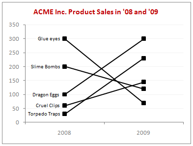
As you can see, interaction plot is a simple line chart with several series. You can easily make this in Excel. Here is a simplified tutorial to help you get started.
Step 1: Select the data and insert a line chart
This is simple, just insert a line chart from the data.
Step 2: Go to the line chart “data” and change rows to columns
You require this step only if your data is oriented differently.

Step 3: Format the interaction chart
Since excel colors each line series differently, you need to change the colors, add labels, adjust the label source (from data to series) and then format grid lines etc.
That is all, your interaction plot is ready to go.
Download interaction plot template for excel and play with it
Click here to download the interaction chart template for excel and use it to make your own interaction plots.
Points to consider when you are making interaction plots,
- Interaction plots can be too messy if you have a lot of series. Generally they loose the appeal after 6-7 series of data.
- Chart formatting with more series of data can be a pain too. Use F4 key if you are found repeating same steps.
- Make sure you don’t color individual series differently. You can use same color and label instead. It looks a lot better that way.
- In cases like last year vs. this year or budget vs. actual, you can even use clustered bars. See more examples on budget vs. actual charts for inspiration.
What is your opinion about interaction plots?
I think they are good for small data samples. I have personally not used them, but I like the idea and will use them when there is an an opportunity. What about you? Have you used them in any professional setting? How did your audience feel about the chart? Tell us using the comments.


23 Responses to “Displaying Text Values in Pivot Tables without VBA”
Its possible to display up to 4 text values.
Have a look at the screen shot of an example that I had posted way back at the EHA and figure out how its done !
http://tinypic.com/r/muzywk/6
With Excel 2010 you can use Conditional Formatting to apply custom number formats which can display text. (In older versions you can only modify text color and cell background color, but not number formats.) Using CF allows for an even larger number of different display values.
[...] Display text values in Pivot Tables without VBA [...]
Hey,
Thanks, this helps. But how do you do it for multiple values where there is a huge amount of non repeating text?
@Soumya
The only way to do more than 4 values is to make the Pivot Table manually with formulas, of course then it isn't a Pivot table
You can of course do it with VBA
You may want to have a look at this description of how to do it here: http://www.clearlyandsimply.com/clearly_and_simply/2011/06/emulate-excel-pivot-tables-with-texts-in-the-value-area-using-vba.html
@Soumya
The only way to do more than 4 values is to make the Pivot Table manually with formulas, of course then it isn’t a Pivot table
You can of course do it with VBA
You may want to have a look at this description of how to do it here: http://www.clearlyandsimply.com/clearly_and_simply/2011/06/emulate-excel-pivot-tables-with-texts-in-the-value-area-using-vba.html
[...] Pivot Tables take tables of data and allow the user to summarise and consolidate the data at the same time. This is a great and very fast method of analysis but is restricted to handling mathematical functions on the value field resulting in numerical summaries. – read more [...]
[…] Read more here: Displaying Text Values in Pivot Tables without VBA […]
There is a very good way actually for handling text inside values area.
First you create a special column on the very left side and call it ID, and put unique ID (numbers only), and then create a pivot table with:
Row Labels and Column labels as you like, and in the Values labels use the unique ID number.
Move the unique ID number (copy paste) somewhere to the right and use vlookup to load the data you need using the ID as reference.
It is a bit longer way but for me it works perfectly to combine values as you like in any moment.
hope helps.
Regards,
Jon
Thank you! I finally understand pivot tables thanks to your clear, concise explanations and examples.
Good Day. This is exactly what i have been looking for. However when i try it on my pivot table or even when i try to recreate this exercise using the sample worksheet, i get this error:
"Microsoft Excel cannot use the number format you typed. Try using one of the built-in number formats."
Same thing here, Excel quite did not like the format in my PowerPivot. Any clues as to what may be going on? Thanks.
I have the same thing happening on my end. I'm running a normal pivot table on a .xlsm file.
@Danzi
What format did you use?
can you post the file ?
pls. help in table there is name, pan. amount. i have to make pivot table for example
NAME PAN AMOUNT
MR.X AAAAC1254T 500.00
MR.Y AAABR1258C
MR.A CFVDE2458T
MR.Z AAVCR12548C
MR.X AAAAC1254T
MR.Z AADCD245T
pls. help in table there is name, pan. amount. i have to make pivot table for example
NAME PAN AMOUNT
MR.X AAAAC1254T 500.00
MR.Y AAABR1258C 1000
MR.A CFVDE2458T 2000
MR.Z AAVCR12548C 5451
MR.X AAAAC1254T 45564
MR.Z AADCD245T 4500
how to get pivot tabe so i get PAN no. against Name.
I found an easy way to get text values in pivot table.
I create an other worksheet in wich each cell has a formula that copy the pivot table. The trick is that the formula does a lookup for the numbers in the pivot table.
The formula looks like that:
=IF(ISNUMBER(table!A1);VLOOKUP(table!A1;Code!$A$1:$B$65;2);IF(ISBLANK(table!A1);" ";table!A1))
Code is a worksheet where there is a liste of text /numbers correspondance.
As a bonus The new sheet is easier to format
Additional trick:
In my case, i encoded differents codeid with a power(2, codeId-1) so that summing then is equivalent to concatenate them.
1-A
2-B
4-C
8-D
yields :
5 - AC
14 - BCD
Hi
I want to ask if pivot can display dates in pivot field. As in a column i have customers and in row different items i want to know there last purchase date. anyone help in this??
Hello Guys, Need your help
I am doing some analysis of the cycle time of the product i.e how much time a product takes from manufacturing to the central warehouse.
I have batch numbers for the product and against them i have to pull out the diff. dates
Like the base date is from where the manufacturing start. So i have the batch number,against it's manuf. date. Now i have to pull out the date when it was quality released.
I have the quality released data but the data have duplicates, like i will have two dates or may be three for the same batch. So my main objective is to pull out the date which is latest among them.
BATCH NO. DATE of Mfg. DATE of Quality release
A1 12/4/2014 (HERE I HAVE TO PULL value)
Next Sheet
BATCH NO. DATE of Quality Release
A1 14/5/2014
a2 23/5/2016
A1 12/5/2014
A1 13/6/2014
From this sheet i have to pull up the latest date format of date here is dd/mm/yyy
TIA
[…] needed to present text instead of counts in a pivot table value column. Here is an excellent resource for Excel manipulation, in addition to an overview of pivot […]
This is great thank you.
Wow!!! Excellent!! It helped me a lot.
I am developing training tracking sheet for 200 employees with training completed date. Each employee will be attending 25 courses. How to indicate actual dates in pivot table value field.