
 Here is a question someone asked me in a class recently.
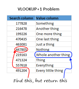
I know how to use VLOOKUP to find a value based on search term. But I have a slight variation to it. I need to extract value below the cell VLOOKUP finds.
This is simpler than it sounds.
We can use INDEX + MATCH formulas to do this.
The syntax is like below:
=INDEX( value column, MATCH (search what, search column, 0) + 1 )
Why it works?
MATCH formula finds the position of what you are searching. By adding 1 to it and extracting the corresponding “values column”, we can get VLOOKUP + 1 value.
Homework for you
If you think finding VLOOKUP+1 is easy then I have a challenge for you.
Find the last match. Lets say in a table you have multiple items matching lookup value. How would you find the last item. Assume what you are finding is in A1, list is in C1:D20 and we want the value in 2nd column.
Go ahead and post your answers in comments section.


41 Responses
This seemed to work for me:
=INDEX(vData,LARGE(IF(vIndex=iValue,ROW(vIndex)),ROW()))
Array entered
vData is the values to pull out, and vIndex is the data to match up, and iValue is the data you’re searching for in cell A1.
Oh, and I guess, so long as you’re pulling numerical/date information out, this should work too:
=SUMPRODUCT(MAX(vIndex=iValue)*(vData))
Oops … missed a set of bracket
=SUMPRODUCT(MAX((vIndex=iValue)*(vData)))
Question is ambiguous — match “below” the key — does that mean the finding the “row located below” the match, or “the next value in ranked-order”, or the “previous value in ranked order”?
11 Apple
33 Pear
55 Corn
22 Banana
44 Orange
66 Grapefruit
If you are looking for “55”, do you want to return (Banana — next one down) or (Grapefruit — next one in ranked order) or (Orange — the one ranked “below” in ranked order)?
I would like to use Array Formula..
`=VLOOKUP(A1,IF($C$1:$C$20=A1,$C$1:$D$20),2,TRUE)`
Regards!
Deb
OOPS.. its in a challenge section.. 🙁
then One more try.. 🙂
=VLOOKUP(LARGE(IF($C$1:$C$20=A1,ROW(D1:D20)),1),IF({1,0},ROW($C$1:$C$20),$D$1:$D$20),2,0)
Array formula:
=INDEX(D:D,MAX(IF(C1:C20=C1,ROW(C1:C20))))
Non-array formula:
=INDEX(D:D,SUMPRODUCT(MAX((C1:C20=C1)*ROW(C1:C20))))
One more array formula:
=LOOKUP(999,IF(C1:C20=A1,ROW(C1:C20)),D1:D20)
A Boolean variation, instead of IF, of Luke’s array formula (plus a typo correction: “=A1”, not “=C1”)
=INDEX(D:D,MAX((C1:C20=A1)*ROW(C1:C20)))
(this is the same Boolean as in his non-array formula)
Chrome crashed so Luke M has beat me to it!
=INDEX(D1:D20,SUMPRODUCT(MAX(–(C1:C20=A1)*(ROW(C1:C20)))))
However I’ve also come up with a formula for returning the nth match (n in A2):
=INDEX($D$1:$D$20,SUMPRODUCT(SMALL(–($C$1:$C$20=$A$1)*(ROW($C$1:$C$20)),COUNTIF(C1:C20,””&A1)+A2)))
Ok that last formula hasn’t come through right there should be in the countif quotes at the end.
Argh (can you tell I don’t post often!), the countif should be:
COUNTIF(C1:C20,”NOT EQUAL TO”&A1)
One more
=LOOKUP(2,1/(C1:C20=A1),D1:D20)
Regards
Amazing Elias. Could you explain be a bit why did you say “2” for lookup value and how 1/(C1:C20=A1) works?
Please explain this!
if we check the series of 1/(C1:C20=A1) the array will be like this:{#DIV/0!;#DIV/0!;1;#DIV/0!;#DIV/0!;#DIV/0!;#DIV/0!;#DIV/0!;#DIV/0!;1;#DIV/0!;#DIV/0!;#DIV/0!;1;#DIV/0!}.
i.e. the maximum value can be 1.9999
lookup of “2” will pick the maximum value among these which is more close to 2.
there is no significance for 2. try any number grater than 2 will give the result.
Jude
Jude — Do you mean the max value in the array can be 1.999? I didn’t get it.
Array-entered:
=OFFSET(D1,MAX((A1=C1:C20)*(ROW(C1:C20)))-1,)
Do these work? I don’t get it. are you meant to be getting the last item value in the D:D column no matter what the value A1 is.
Kevin, are you asking me? If so, yes my formula works. It returns the last value in range D1:D20 when value in range C1:C20 is equal to A1.
Regards
“Max-If” approach with a third column (F). Formula is in B2.
=INDEX($D$2:$D$23,MAX(IF($C$2:$C$23=A2,$E$2:$E$23)),1)
CHALLENGING ONE
=INDEX($D$1:$D$20,SUMPRODUCT(MAX(((C1:C20=A1)*1)*ROW(C1:C20))))
Although I think many people beat me to this! 🙂
dont know the answer, can’t wait to see it pusblished, I do have a challenge right now with this exact scenario where I need to find the last value associated to a match value
Ladies/Gents,
Appreciate all these formula inputs; chandoo must be having a tough time house keeping these comment session.
Let’s try this way.
Sample table:-
A 40000
B 3
c 4
C 5
c 89
C 45
d 7
Sort the table in ascending order
With the table in ascending order, the last parameter will give you the two different results:
VLOOKUP(“C”, table_name, 2, 1) returns the last match, 45
VLOOKUP(“C”, table_name, 2, 0) returns the first match, 4
Isn’t that the simplest option?(IF you can sort parent table data)..
Otherwise I would certainly go with Elias(But the Q was to use VLOOOKUP and not LOOKUP)
Dear Microsoft..world is evolving.. requirements are changing and challenging ..why don’t you guys introduce vlookup2.0..which is smart enough to hunt and grab the Nth value in a table unlike the current one which picks only the boring first value?..my dream vlookup2.0 would look like…VLOOKUP2(this value, in this list, and get me value in this column, [is-my-list-sorted?, Nth Position)..hope to see soon 🙂
I think the question/challenge is asking to match the value in a1 with the values in range c1:c20 and return the value of next row from range d1:d20. If my understanding is correct then this formula works well ‘=INDEX(D1:D20,MATCH(A1,C1:C20,0)+1)’
i’m with Raza. the other formulas seem to be giving the results of the same rows. since he already provided the same solution i’m thinking, here’s another:
=VLOOKUP(A1,CHOOSE({1,2},C1:C20,D2:D21),2,0)
missed the portion where it has multiple values. this would help:
=LOOKUP(A1,1/(C1:C20=A1),D2:D21)
Hello, what a nice post!
Simply trying to apply this vlookup+1 to a multi-sheet case.
My syntax gives error:
=+INDEX(Sheet2!Where_to_look;MATCH(Sheet1!Ref_Iam_searching;Sheet1whole column;0)+1)
Anyone for a solution? Thanks!
I used a ‘helper’ column in column E with formula:
=C2&COUNTIF($C$2:C2,C2)
Then used index formula as follow:
=INDEX(D1:D20,MATCH(A1&COUNTIF(C1:C20,A1),E1:E20,0))
Dear Chandoo,
00.00.0002
00.02.0001
01.02.0000
The answer is 01.04.0003 if add. How to add the above three values. Please furnish the formula.
Thank you sir
@Kattekola
Are these cells text or numbers ?
@Kattekola
Actually just try
=TEXT(SUMPRODUCT(–LEFT(A1:A3,2)),”00″)&”.”&TEXT(SUMPRODUCT(–MID(A1:A3,4,2)),”00″)&”.”&TEXT(SUMPRODUCT(–RIGHT(A1:A3,2)),”0000″)
If you copy/paste this formula retype the ” marks manually
Sheet1 Sheet2
ID type id 1 MONTH type Jan13 DATA
NAME Disply Name INDIA ID NAME Month Value1 Value2
1 INDIA JAN13 252 357
2 China FEB13 25 95
Value 1 Display Value as 252
Value 2 357
Dude, thanks, that was awesome and simple!
=INDEX($A$2:$C$5,MATCH(A2,$A$2:$A$5,0)+1,3)
Sr B R
1 40 28
2 50 36
3 63 45
4 80 45
5 80 56
6 100 56
With respect to the above example, I am trying to do the following,
– The user has to input one value of ‘B’ and one value for ‘R’ only in the above combinations of ‘B’ and ‘R’. For Eg. If ‘B’=40, ‘R’ can only be 28. However if ‘B’ is 80, ‘R’ can be either 45 or 56.
-If ‘B’ is 80 and ‘R’ is 45, I want the value returned to be 4. However if ‘B’ is 80 and ‘R’ is 56, I want the value 5 to be returned. If ‘B’ is 63 and ‘R’ is 56, return a error as this combination is not one of the pairs above.
Please help!
Definitely, what a great website and enlightening posts, I definitely will
bookmark your blog.Best Regards!
Such a helpful website. I went through all the replies however I think my question is a bit more unique.
I’ve got dates as seen below:
QTR 1 QTR 2 QTR 3
2016 Q2 2016 Q3 2016 Q4
I need a formula that when you input QTR1, the result is 2016Q2. I am struggling to get this to work. I’ve used Index Match and others.
When I use the formula below, assuming QTR 2, I get the result of 2016 Q2
This thread is very helpful. My request is a bit unique. I have the following data set.
ACTIVEQTR1 ACTIVEQTR2 ACTIVEQTR3 ACTIVEQTR4
Q1 2016_Units Q2 2016_Units Q3 2016_Units Q4 2016_Units
I have a blank field for which I entered ACTIVEQTR2. And I need a formula that will spit out Q2 2016_Units based on the ACTIVEQTR2 input. How would I go about that. I tried the following formula:
=INDEX(AB2:AE2,SUMPRODUCT(MAX(–(AB1:AE1=AC23)*(ROW(AB1:AE1)))))
Unfortunately the above formula when using ACTIVEQTR2 as my input spits out Q1 2016_Units instead of Q2 2016_units.
Help!