
Hi folks…
Are you ready for an Excel challenge?
Today, your job is very simple. Just find a pattern in a text and return corresponding value.
Your Homework:
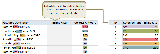
In a range we have some resource types & their billing rates.
In another range, we have some descriptions. Each description contains a resource type somewhere inside it. We need to retrieve billing rate for each description by looking up which resource type is mentioned in it.
See this diagram:
Download the data
Click here to download the data to write your formulas.
Notes:
- The file contains 3 named ranges – resIDs, resTypes, resRates for resource IDs, types & rates in that order. You can use these to shorten your formulas.
Post your answers:
Go ahead and solve this. Then come back and post your formulas in comments. Click here to post your answer.
Need clues?
Read wildcards in COUNTIF formula page to get some clues.
So go ahead and post your answers. I am waiting…


240 Responses
Not my formula but this will do the trick…
=LOOKUP(2^15,SEARCH(resTypes,B4),resRates)
~VijaySharma
Great solution! Trying to figure out how it works. Could you explain? especially the 2^15 part.
Peter
Seems like here might be an answer:
http://www.youtube.com/watch?v=huDPpuOucF0
The 2^15 is the lookup value and needs to be large enough to be greater then the length of the text in B4, since the search function will return #VALUE! for the search terms not matched and the position of the matched search term.
Effectively, the lookup becomes =LOOKUP(2^15,{#VALUE!;#VALUE!;#VALUE!;9;#VALUE!;#VALUE!},resRates)
2^15 is an arbitrary number for this example. The largest position that SEARCH returns in this example is 16, which can be used in the example.
This formula works unless you have a Resource Description of “FM Radio Station AM xxxxx2324” or anything combination before the resource type that matches a different resource type. So in my example there is FM which is not the type in this description but the formula will still pick it up as the type and bring back a 75 instead of a 50.
I love this one however it fails if some string appears in a word
I would add a trailing space (and leading ?).
=LOOKUP(2^15;SEARCH( esTypes & ” “;B4);resRates)
Then you can use this one…
=LOOKUP(2^15,SEARCH(resTypes & ” xxx”, B4 & ” xxx”), resRates)
That’s close, I think. But if there is a couple of research types like PM and PPM then you’d still get the wrong answer.
<code>=LOOKUP(2^15, SEARCH(” ” & resTypes & ” “, B4), resRates)</code>
I think this’d take care of it.
Almost 🙂
=LOOKUP(2^15,SEARCH(” ” & resTypes & ” xxx”, ” ” & B4 & ” xxx”), resRates)
Uuups, no you are right…
in fact the best & right answer
array formula
=VLOOKUP(INDEX($H$4:$H$9,MAX(IF(ISERROR(FIND($H$4:$H$9,B4)),-1,1)*(ROW($H$4:$H$9)-ROW($H$4)+1))),$H$4:$I$9,2,FALSE)
Love this formula, agree with Irvine, 2^15 can be replaced with any number as long as it is similar or has greater length than the text on column B.
with addition of index and match it can help you find the correct billing rate.
It is working for LOOKUP, But if I am trying with VLOOKUP it is not working. Any idea why?
This works too:
=LOOKUP(1000,SEARCH(resTypes,B4),resRates)
First I used replace function to free resource type with not required text and value, then used v look formula to get the billing rate Resource Description Billing Rate Correct Answers
Nothing CM xxxx4607 CM 120 120
Few things CXO xxxx5633 CXO 250 250
Lots of things RM xxxxxx6378 RM 150 150
Something AM xxxx9132 AM 50 50
One thing AM xxx5299 AM 50 50
Few things PM xxxxx5502 PM 60 60
Nothing AM xxxx6096 AM 50 50
Another thing RM xxx7837 RM 150 150
Something AM xxxxx6719 AM 50 50
One thing FM xxx1817 FM 75 75
One thing CXO xxxxx2823 CXO 250 250
Nothing AM xxx5155 AM 50 50
Another thing FM xxxx3012 FM 75 75
Something AM xxx2124 AM 50 50
Nothing CM xxxx9363 CM 120 120
One thing CM xxxx2104 CM 120 120
Nothing FM xxxxx1386 FM 75 75
Another thing PM xxx9637 PM 60 60
Few things PM xxxx8157 PM 60 60
One thing PM xxxxxx9699 PM 60 60
Few things RM xxxxxx8637 RM 150 150
Lots of things RM xxxxxx3863 RM 150 150
Something CM xxxxx4671 CM 120 120
One thing CXO xxxx2450 CXO 250 250
Nothing PM xxxx1759 PM 60 60
Something RM xxxx8382 RM 150 150
Something PM xxxxxx8054 PM 60 60
Another thing CXO xxxx1293 CXO 250 250
Something RM xxx4545 RM 150 150
Something RM xxxxxx7317 RM 150 150
=XLOOKUP(TRUE, ISNUMBER(SEARCH(resTypes, B4)), resRates, “Not Found”)
=RECHERCHEV(SUPPRESPACE(DROITE(GAUCHE(B4;TROUVE(“xx”;B4)-2);3));$H$4:$I$9;2;0)
=Vlookup(trim(right(left(b4;find(“xx”;b4)-2);3));$h$4:$i$9;2;0)
cant replace right(left()) with a stxt()
Formula is too long but it works
=VLOOKUP(MID(B4,IF(ISERROR(FIND(“ngs”,B4)),FIND(“ng”,B4)+3,FIND(“ngs”,B4)+4),2)&”*”,$H$4:$I$9,2,0)
~lilg
What i’ve figured out is:
{=INDEX(resRates;SUM(NOT(ISERROR(SEARCH(resTypes;B4;1)))*ROW(resTypes))-3)}
Here is my solution (array formula):
INDEX(resRates,MATCH(0,FIND(resTypes,B4,1)*($J$4:$J$9),0))
Hi,
I have used countif & If conditions, Please do let me know if we have any other better way…
IF(COUNTIF(B4,”*”&$H$4&”*”)<>0,$I$4,IF(COUNTIF(B4,”*”&$H$5&”*”)<>0,$I$5,IF(COUNTIF(B4,”*”&$H$6&”*”)<>0,$I$6,IF(COUNTIF(B4,”*”&$H$7&”*”)<>0,$I$7,IF(COUNTIF(B4,”*”&$H$8&”*”)<>0,$I$8,IF(COUNTIF(B4,”*”&$H$9&”*”)<>0,$I$9,”Check”))))))
Looking forward to learn a lot from here…..
Cheers…
1. INDEX(resRates,MATCH(1,–(ISNUMBER(FIND(resTypes,B4))),0))
2. INDEX(resRates,SMALL(IF(1*(ISNUMBER(FIND(resTypes,B4))),ROW(resTypes)-ROW($H$4)+1),1))
Both required Ctrl+shift+Enter
I like Vijay’s best so far, but this is what I first came up with. Maybe I just love using SUMPRODUCT too much….
=SUMPRODUCT(ISNUMBER(SEARCH(resTypes,B4))*(resRates))
Yes Luke You Do Love Very much of Sumproduct
sumproduct is useful function which was developed by excel user like us…and idea apply by MS in excel 2007 as sumifs……:D
GFC variation :
=RECHERCHEV(SUBSTITUE(DROITE(GAUCHE(B4;CHERCHE(“xx”;B4)-2);3);” “;””);$H$3:$I$9;2;0)
array formula
=SUM((IFERROR(SEARCH(resTypes,b4),0)<>0)*resRates)
I too like Vijay’s LOOKUP formula since it very short and to the point!
(I would wrap the restypes in a space on either side to avoid any false positives.)
Here is what I came up with:
=INDEX(resRates, MATCH(99,FIND(” ” & resTypes & ” “, B4)))
Ctrl + Shift + Enter
The idea is similar to a few of the formulas already posted.
Cheers,
Sajan.
Looks like I’m the only one that went the vba route with this one. I think I got a good handle on formulas since been using them since forever, so always look for ways to improve my vba skills. Well anyways, here it is.
https://www.dropbox.com/s/qipm1hoczmvrxgv/can-you-find-the-pattern%20NMone.xlsm
=OFFSET(resRates,MAX((IFERROR(FIND(resTypes,B4,1),0)>1)*resIDs)-1,0,1,1)
=OFFSET(resRates,MAX((IFERROR(FIND(resTypes,B4,1),0)>1)*resIDs)-1,0,1,1)
Ctrl+Shift+Enter of course.
=VLOOKUP(TRIM(CLEAN(RIGHT(MID(B4,1,FIND(“x”,B4)-1),4))),$H$3:$I$9,2,0)
=IF(NOT(ISERROR(SEARCH($H$4,B4))),$I$4,IF(NOT(ISERROR(SEARCH($H$5,B4))),$I$5,IF(NOT(ISERROR(SEARCH($H$6,B4))),$I$6,IF(NOT(ISERROR(SEARCH($H$7,B4))),$I$7,IF(NOT(ISERROR(SEARCH($H$8,B4))),$I$8,IF(NOT(ISERROR(SEARCH($H$9,B4))),$I$9))))))
=INDEX(resRates,MATCH(TRIM(LEFT(RIGHT(B4,LEN(B4)-FIND(” x”,B4)+4),3)),resTypes,0),1)
=SUMPRODUCT(COUNTIF(B4,”*”&resTypes&”*”)*resRates)
Assign a code relevant to match with resource type in column A by filtering text contain resource type……then use simple forlmula…. =VLOOKUP(A4,$H$4:$I$9,2,FALSE) …
=VLOOKUP(SUBSTITUTE(MID(B4,FIND(“x”,B4,1)-4,3),” “,””),$H$4:$I$9,2,0)
Awesome nonfancy formula
Two solutions.
=LOOKUP(2,1/COUNTIF(B4,”*”&resTypes&”*”),resRates)
=LOOKUP(9^9,SEARCH(resTypes,B4),resRates)
=VLOOKUP(TRIM(MID(B4,FIND(“x”,B4,1)-4,3)),$H$4:$I$9,2,FALSE)
=SUMPRODUCT(1-ISERROR(FIND(resTypes,B4)),resRates)
Good answer..elegant solution. So, by using the Sumproduct function, the Find function can handle an array of values that it normally could not do outside of the Sumproduct function??? Thanks for the post.
I couldn’t figure out how to do it without a “helper” column, (I kept running into errors when I tried to nest VLOOKUP. So I just created a nested IF formula in the E column to tell me the resource’s ID:
=IF(ISNUMBER(FIND(“AM”,B4)),1,IF(ISNUMBER(FIND(“PM”,B4)),2,IF . . . etc.
Then, I just used a simple VLOOKUP with a reference to the ID in column E:
=VLOOKUP(E4,$G$4:$I$9,3)
Not the most elegant solution. I’m looking forward reading the awesome that all of you used to solve this.
=SUMPRODUCT(–(TRIM(MID(B4,FIND(“x”,B4)-4,3))=(resTypes)),resRates)
Similar to others looking left of x’s
=VLOOKUP((TRIM(MID(B4,TRIM(FIND(“x”,B4,1)-4),3))),$h$4:$i$9,2,FALSE)
=IF(COUNTIF(B4,”*CM*”)=1,VLOOKUP(4,RANGE1,3,FALSE),(IF(COUNTIF(B4,”*CXO*”)=1,VLOOKUP(6,RANGE1,3,FALSE),(IF(COUNTIF(B4,”*RM*”)=1,VLOOKUP(5,RANGE1,3,FALSE),(IF(COUNTIF(B4,”*AM*”)=1,VLOOKUP(1,RANGE1,3,FALSE),(IF(COUNTIF(B4,”*PM*”)=1,VLOOKUP(2,RANGE1,3,FALSE),(IF(COUNTIF(B4,”*FM*”)=1,VLOOKUP(3,RANGE1,3,FALSE))))))))))))
very elegant!
Haha, far from pretty, far from elegant, and FAR from dynamic, but it works:
=IF(NOT(ISERROR(FIND($H$4,$B4,1))),$I$4,IF(NOT(ISERROR(FIND($H$5,$B4,1))),$I$5,IF(NOT(ISERROR(FIND($H$6,$B4,1))),$I$6,IF(NOT(ISERROR(FIND($H$7,$B4,1))),$I$7,IF(NOT(ISERROR(FIND($H$8,$B4,1))),$I$8,IF(NOT(ISERROR(FIND($H$9,$B4,1))),$I$9,”N/A”))))))
Man, all of you guys’ other answers are quite impressive. Mine I thought was pretty simple, yet works perfectly. Let me know what you think…
=IFERROR( INDEX( resRates, MATCH( MID( B4, (FIND( “M”, B4) -1), 2), resTypes, 0), 1), 250)
Took two approaches
1. created a separate table setting the “Resource Type” than using that table for VLOOKUP reference
TRIM(CLEAN(MID(B4,FIND(“x”,B4)-4,3)))
followed by
IFERROR(VLOOKUP(L4,rate,2,FALSE),””)
OR….
2. A singular VLOOKUP combining efforts:
=IFERROR(VLOOKUP((TRIM(CLEAN(MID(B4,FIND(“x”,B4)-4,3)))),rate,2,FALSE),””)
Thank you that was fun.
=SUM(resRates*COUNTIF(B4,”*”&resTypes&”*”))
Array entered
WOOOOW!!!!
Mike,
LOVE IT, LOVE IT,,simplicity
Looks simples, but I get zero for value when I plug the formula into cell C4 and down. Anyone else has that problem?
Even I am getting Zero when i plug the same formula in C4.
Can you assist?
Please explain this formula…mainly about array
I exploited the commonality of the resource desc field values, and then did a little bit trial and error… with “things” and “thing” there are some offshoot of number of characters, fortunately you have spacebar in between thing/things and xxx… thus trim worked.
=VLOOKUP(TRIM(MID(B4,FIND(“thing”,B4,1)+LEN(“thing”)+1,FIND(“x”,B4,1)-FIND(“thing”,B4,1)-LEN(“thing”)-2)),$H$3:$I$9,2,FALSE)
Thanks, Somak
Excellent answers everyone… Here is my solution.
{=INDEX(resRates,MAX(COUNTIF(B4,”*”&resTypes&”*”)*(resIDs)))}
Solution file.
Why not just this array-entered formula without the INDEX part?
=MAX(COUNTIF(B4,”*”&resTypes&”*”)*resRates)
Really good suggestion, Rick, but I think it only works if all array elements are numeric. If result is non-numeric then INDEX or something similar will be needed.
I got answer…
{=VLOOKUP(“*CM*”,H4:I9,2,0)}
If there is no match the result is wrong (for example: Description “Few things xxxx5633”, gives the answer: 50
There is no AF In this description.
That because we get a zero vector to maximize.
=IF(COUNTIF(B4,”*M*”),VLOOKUP(MID(B4,FIND(“M”,B4)-1,2),$H$4:$I$8,2,0),$I$9)
There was a similar case on Chandoo forum.
Here it is:
http://chandoo.org/forums/topic/search-for-a-word-string-and-return-that-string-if-found
=INDEX($H$4:$I$9,MATCH(MID(SUBSTITUTE(B5,” “,”@”,LEN(B5)-LEN(SUBSTITUTE(B5,” “,””))-1),SEARCH(“@”,SUBSTITUTE(B5,” “,”@”,LEN(B5)-LEN(SUBSTITUTE(B5,” “,””))-1))+1,SEARCH(” “,SUBSTITUTE(B5,” “,”@”,LEN(B5)-LEN(SUBSTITUTE(B5,” “,””))-1),SEARCH(“@”,SUBSTITUTE(B5,” “,”@”,LEN(B5)-LEN(SUBSTITUTE(B5,” “,””))-1)))-SEARCH(“@”,SUBSTITUTE(B5,” “,”@”,LEN(B5)-LEN(SUBSTITUTE(B5,” “,””))-1))-1),resTypes,0),2)
SUMP RODUCT IS SIMPLEST
HI
I have taken Combination of Left, Right,Find & Trim with VLookup
=VLOOKUP(TRIM(RIGHT(LEFT(B4,FIND(” x”,B4)-1),3)),$H$4:$I$9,2,0)
i am totally agree with Vijay Shrama solution. Here is i am explaining the trick
=LOOKUP(16,SEARCH(resTypes,B4),resRates)
The text length of starting CM,AM etc is maximum 16, so this formula works also by putting 16. Any how if you not now the length than the best maximum digit should be enter.
Dear Chandoo
you are working really awesome, i am in very initial stage. i like your tricks. I started Excel about 8 months ago. From your blog and Mr, Excel is fun i have learned a lot.
also i request you if you will guide me how can i improve my self.
Thanks & Regards
Muhammad Shakeel
is the simple and best…….
Description
LEN
Nothing C
9
Few things P
12
Lots of things A
16
Something P
11
One thing A
11
Another thing C
15
correction
Description LEN
Nothing C 9
Few things P 12
Lots of things A 16
Something P 11
One thing A 11
Another thing C 15
Hi everyone,
May I suggest the following array formula :
{=INDEX(resRates,MAX(ISNUMBER(IFERROR(FIND(” ” & resTypes & ” “,B4),””))*resIDs))}
As you could notice :
I did not use any wild card.
I supposed the ‘codes’ were had no blank space in front and/or behind (e.g. CM, not [ CM], [ CM ] or [CM ]
I wanted to avoid that any code could be found inside another word (in col B)
I finally could find the trick to get it work whatever the length of the code
Congratulations and Thanks to you all
Have a great week end
A Frenchie
=VLOOKUP(“*”&H4&”*”,$B$3:$D$33,3,0)
=MAX(IFERROR((SEARCH(“*”&resTypes&”*”,B4))*1*(resRates),0))
=VLOOKUP(TRIM(MID(B4,LARGE(IF(MID(B4,ROW($A$1:$A$50),1)=” “,ROW($A$1:$A$50),0),2)+1,3)),$H$4:$I$9,2,0)
Array-entered.
Meanwhile Waiting
Hi again,
Here’s another suggestion
=INDEX(resRates,SUM(–ISNUMERIC(FIND(” ” & resTypes & ” “,B4))*resIDs))
As an array formula (CTRL+SHIFT+Enter)
Seems to work well …
=MAX(IFERROR((SEARCH(resTypes;B4)/SEARCH(resTypes;B4))*resRates;0))
Hi
using with array formula
=MAX(IFERROR(SEARCH(resTypes,B4)/SEARCH(resTypes,B4)*(resRates),0))
CTR+SHFT+ENTER
Not working
This one as well:
=INDEX(resRates,SUM(IF(IFERROR((SEARCH(resTypes,B4)*ROW($A$1:$A$6))>0,0),ROW($A$1:$A$6))),0)
Ctrl+Shift+Enter
Regards,
Hi All,
This one as well:
=INDEX(resRates,SUM(IF(IFERROR((SEARCH(resTypes,B4)*ROW($A$1:$A$6))>0,0),ROW($A$1:$A$6))),0)
Hi
This one as well
=INDEX(resRates,SUM(IF(IFERROR((SEARCH(resTypes,B4)*ROW($A$1:$A$6))>0,0),ROW($A$1:$A$6))),0)
=VLOOKUP(TRIM(MID(B4,FIND(“x”,B4)-4,3)),$H$4:$I$9,2,0)
{=SUMPRODUCT(IF(IFERROR(FIND($H$4:$H$9;B4);0)>0;1;0);$I$4:$I$9)}
=VLOOKUP(TRIM(MID(B4,FIND(” x”,B4,1)-3,3)),$H$4:$I$9,2,FALSE)
Came up with this in a couple min. It works but it’s not as generic as I’d like.
I ended up with the following array formula
=SUMPRODUCT(IF(ISNUMBER(FIND(resTypes,B28))=TRUE,1,0),resRates)
This will work:
=LOOKUP(2^10,SEARCH(resTypes,B4),resRates)
Request you to explain about 2^10
I came up with this… I see many have similar entries
=SUMPRODUCT(IF(IFERROR(FIND(resTypes,B4),0)=0,0,1)*resRates)
One thing I would suggest to people who have used SEARCH in their formula. SEARCH isnt case-sensitive so in a case like this, it would be better to use FIND.
I have got the correct results, the following is the formula :
VLOOKUP(TRIM(IF(ISERROR(IF(ISERROR(MID(B4,FIND(” “,B4,FIND(” “,B4,FIND(” “,B4,1)+1)+1)+1,FIND(” “,B4,FIND(” “,B4,FIND(” “,B4,FIND(” “,B4,1)+1)+1)+1)-FIND(” “,B4,FIND(” “,B4,FIND(” “,B4,1)+1)+1))=TRUE),MID(B4,L4+1,FIND(” “,B4,FIND(” “,B4,FIND(” “,B4,1)+1)+1)-FIND(” “,B4,FIND(” “,B4,1)+1)),MID(B4,FIND(” “,B4,FIND(” “,B4,FIND(” “,B4,1)+1)+1)+1,FIND(” “,B4,FIND(” “,B4,FIND(” “,B4,FIND(” “,B4,1)+1)+1)+1)-FIND(” “,B4,FIND(” “,B4,FIND(” “,B4,1)+1)+1)))=TRUE),MID(B4,FIND(” “,B4,1)+1,FIND(” “,B4,FIND(” “,B4,1)+1)-FIND(” “,B4,1)),IF(ISERROR(MID(B4,FIND(” “,B4,FIND(” “,B4,FIND(” “,B4,1)+1)+1)+1,FIND(” “,B4,FIND(” “,B4,FIND(” “,B4,FIND(” “,B4,1)+1)+1)+1)-FIND(” “,B4,FIND(” “,B4,FIND(” “,B4,1)+1)+1))=TRUE),MID(B4,FIND(” “,B4,FIND(” “,B4,1)+1)+1,FIND(” “,B4,FIND(” “,B4,FIND(” “,B4,1)+1)+1)-FIND(” “,B4,FIND(” “,B4,1)+1)),MID(B4,FIND(” “,B4,FIND(” “,B4,FIND(” “,B4,1)+1)+1)+1,FIND(” “,B4,FIND(” “,B4,FIND(” “,B4,FIND(” “,B4,1)+1)+1)+1)-FIND(” “,B4,FIND(” “,B4,FIND(” “,B4,1)+1)+1))))),$H$4:$I$9,2,0)
I got it, following is the formula :
=VLOOKUP(TRIM(IF(ISERROR(IF(ISERROR(MID(B4,FIND(” “,B4,FIND(” “,B4,FIND(” “,B4,1)+1)+1)+1,FIND(” “,B4,FIND(” “,B4,FIND(” “,B4,FIND(” “,B4,1)+1)+1)+1)-FIND(” “,B4,FIND(” “,B4,FIND(” “,B4,1)+1)+1))=TRUE),MID(B4,L4+1,FIND(” “,B4,FIND(” “,B4,FIND(” “,B4,1)+1)+1)-FIND(” “,B4,FIND(” “,B4,1)+1)),MID(B4,FIND(” “,B4,FIND(” “,B4,FIND(” “,B4,1)+1)+1)+1,FIND(” “,B4,FIND(” “,B4,FIND(” “,B4,FIND(” “,B4,1)+1)+1)+1)-FIND(” “,B4,FIND(” “,B4,FIND(” “,B4,1)+1)+1)))=TRUE),MID(B4,FIND(” “,B4,1)+1,FIND(” “,B4,FIND(” “,B4,1)+1)-FIND(” “,B4,1)),IF(ISERROR(MID(B4,FIND(” “,B4,FIND(” “,B4,FIND(” “,B4,1)+1)+1)+1,FIND(” “,B4,FIND(” “,B4,FIND(” “,B4,FIND(” “,B4,1)+1)+1)+1)-FIND(” “,B4,FIND(” “,B4,FIND(” “,B4,1)+1)+1))=TRUE),MID(B4,FIND(” “,B4,FIND(” “,B4,1)+1)+1,FIND(” “,B4,FIND(” “,B4,FIND(” “,B4,1)+1)+1)-FIND(” “,B4,FIND(” “,B4,1)+1)),MID(B4,FIND(” “,B4,FIND(” “,B4,FIND(” “,B4,1)+1)+1)+1,FIND(” “,B4,FIND(” “,B4,FIND(” “,B4,FIND(” “,B4,1)+1)+1)+1)-FIND(” “,B4,FIND(” “,B4,FIND(” “,B4,1)+1)+1))))),$H$4:$I$9,2,0)
=TRIM(MID(B4,IFERROR(IFERROR(IFERROR(SEARCH((“ing ?? xx”),B4)+5,SEARCH((“ings ?? xx”),B4)+5),SEARCH((“ing ??? xx”),B4)+5),SEARCH((“ings ??? xx”),B4)+5)-1,SEARCH(“xx”,B4)-IFERROR(IFERROR(IFERROR(SEARCH((“ing ?? xx”),B4)+5,SEARCH((“ings ?? xx”),B4)+5),SEARCH((“ing ??? xx”),B4)+5),SEARCH((“ings ??? xx”),B4)+5)))
my solution is also long 🙁
=VLOOKUP(IF(MID(B4,FIND(“x”,B4)-1-3,1)=” “,MID(B4,FIND(“x”,B4)-1-2,2),MID(B4,FIND(“x”,B4)-1-3,3)),$H$3:$I$9,2,0)
=INDEX(resRates,MATCH(TRUE,IFERROR(FIND(resTypes,B5),0)<>0,0))
Ctrl+Shift+Enter for array formula
Hi chandoo,
although i havent use countif function, but i have found an alternative to this problem. my only concern is that it took me 15-20 mins atleast for arriving at this solution which to too much. if u cud sugest a shorter or more simpler solution to it, i shall be grateful.
=VLOOKUP(IF(MID(B8,FIND(“x”,B8)-4,1)=” “,MID(B8,FIND(“x”,B8)-3,2),MID(B8,FIND(“x”,B8)-4,3)),$H$3:$I$9,2,0)
Hi chandoo,
although i havent use countif function, but i have found an alternative to this problem. my only concern is that it took me 15-20 mins atleast for arriving at this solution which to too much. if u cud sugest a shorter or more simpler solution to it, i shall be grateful.
Late to the party but here is what I came up with
=MAX(IFERROR(MATCH(“*”&$H$4:$H$9&”*”,B4,0),0)*resRates)
Entered as an array:
=VLOOKUP(MATCH(1,COUNTIF(B4,”*”&resTypes&”*”),0),$G$4:$I$9,3,0)
Not as elegant/straightforward as some of the others, but does not rely on the entry of an arbitrarily large value like 2^15.
Quite late though , This formula gave me desired result :
=VLOOKUP(TRIM(IF(FIND(“ing”,B4,1),MID(B4,IFERROR(FIND(“ings”,B4,1),FIND(“ing”,B4,1))+4,FIND(” x”,B4)-(IFERROR(FIND(“ings”,B4,1),FIND(“ing”,B4,1))+4)),IF(FIND(“ings”,B4,1),MID(B4,IFERROR(FIND(“ings”,B4,1),FIND(“ing”,B4,1))+5,FIND(” x”,B4)-(IFERROR(FIND(“ings”,B4,1),FIND(“ing”,B4,1))+5))))),$H$4:$I$9,2,0)
=VLOOKUP(TRIM(RIGHT(LEFT(B4,FIND(” xxx”,B4,1)),4)),$H$4:$I$9,2,FALSE)
hi,
TO Vijay:
Is it mendatory to put 2^15.
if i want to try with another string.
i.e.
PJEAL-S-JY13551-12A1
In that string i want 12a1.
no doubt with your formula i m getting result. but i want to understand the fundamental about “2^15”.
Hope you will understand.
Regards
Istiyak
You don’t need to use 2^15. You just need to use a number that is bigger than the size (number of characters) of your largest string. If your strings are always less than 30 characters, you can use 30 instead of 2^15. If you don’t know the size of your strings or you want to use a number that fits all situations, use the max number of characters a cell can hold (which is 32768 = 2^15).
=VLOOKUP(TRIM(MID(B4,FIND(“x”,B4)-4,4)),$G$4:$H$9,2,FALSE)
where B4 is the search string, and $G$4:$H$9 is the vlookup range.
Hey I tried this long formula and it worked VLOOKUP(IF(COUNTIF(B4,”*”&$H$4&”*”)<>0,$H$4,IF(COUNTIF(B4,”*”&$H$5&”*”)<>0,$H$5,IF(COUNTIF(B4,”*”&$H$6&”*”)<>0,$H$6,IF(COUNTIF(B4,”*”&$H$7&”*”)<>0,$H$7,IF(COUNTI………………..
my answer is
=VLOOKUP((TRIM(RIGHT((LEFT(B4,FIND(” x”,B4))),4))),$H$4:$I$9,2,0)
=IF(ISERROR(FIND(H$4,B4)),IF(ISERROR(FIND(H$5,B4)),IF(ISERROR(FIND(H$6,B4)),IF(ISERROR(FIND(H$7,B4)),IF(ISERROR(FIND(H$8,B4)),IF(ISERROR(FIND(H$9,B4)),0,250),150),120),75),60),50)
Please display the full formula
Hi Chandoo
Loved this post!
I find these days, I immediately default to using Boolean logic when dealing with array formulas – especially as the COUNTIF first argument “range” doesn’t accept arrays – BUT I did not know that the second argument can!
So here is my formula:
=INDEX(resRates,MATCH(1,COUNTIF(B4,”*”&resTypes&”*”),0))
Thanks for the great content
=LOOKUP(9.99999999999999E+307,SEARCH(resTypes,B4),resRates)
Being in the E-Commerce Industry, I use this awesome trick all the time to get the color of the products form there names from a list of colors.
Having said that the problem with this formula is that it would look up the keywords inside a word or any where in the text also for example the keyword “AM” would be looked up in the following sentence “NoAMing CM xxxx4607″ (just for eg.) but the correct answer should be CM instead of AM. To avoid this what I do is add a space before and after the keyword, which reduces the chances of this kind of errors.
Hi,
i used below formula & got the answers
=VLOOKUP(TRIM(RIGHT(LEFT(B4,FIND(“xxx”,B4,1)-2),3)),$H$4:$I$9,2,0)
Building the 2 char code:
=RIGHT(LEFT(B4,FIND(“x”,B4)-2),2)
find the wildcard code via vlookup:
=VLOOKUP(“*”&E4&”*”,$H$4:$I$9,2,0)
of course you can join them together. ( but it harder to understand )
E4 IN the previous is the 2 char code.
Haven’t seen my solution here yet:
{=SUM(IF(ISERROR(FIND(resTypes,B2)),0,resRates))}
This is an array formula. Enter it without the curly braces and hit Ctrl+Shift+Enter instead of Enter.
can some body explain me, =SEARCH(resTypes,B4) as it returns # VALUE! in my excel sheet
@Usman
It’s because the value in B4 can’t be found in the Range resTypes
This is either because B4 isn’t in the range or that the range isn’t where you think it is
You may also want to check that either B4 or the values in the range don’t have leading or trailing spaces
@Hui thanks, I guess u have answers to my questions 🙂
the thing is vijay posted this formula (above) =LOOKUP(16,SEARCH(resTypes,B4),resRates)
what I am trying is to understand is that how this formula works so I took out the SEARCH(resTypes,B4) part out to understand in pieces but it returns #VALUE! so I m confused, and one more thing is it necessary for the search formula refer to a named range or I can give simple range like H4:H9 ???
please help and thanks alot 🙂
@Usman
It depends on where the name ResTypes is referring to are you sure it’s where you expect?
Can you post the file?
I dont no how to post file ? as there is isnt any link for uploading file can i email u or some thing…..as I also want to send u the file for the Question on sum product that we have been discussing on another page.
@Usman
You can email me click on Hui… above or
http://chandoo.org/forums/topic/posting-a-sample-workbook
Well, here is my solution:
=SUMPRODUCT(COUNTIF(B4,”* “&resTypes&” *”),resRates)
by entering an array in COUNTIF function I get back an array of same size as resType consisting of 1s and 0s. So, I used that array to multiply the billing rate array using SUMPRODUCT. Brilliant website, makes the complicated understandable.
=VLOOKUP(TRIM(RIGHT(MID(B4,1,FIND(” x”,B4,1)),4)),$G$4:$H$9,2,FALSE)
=IF(ISNUMBER(FIND(“CM”,B5)),$I$7,IF(ISNUMBER(FIND(“PM”,B5)),$I$5,IF(ISNUMBER(FIND(“FM”,B5)),$I$6,IF(ISNUMBER(FIND(“AM”,B5)),$I$4,IF(ISNUMBER(FIND(“RM”,B5)),$I$8,IF(ISNUMBER(FIND(“CXO”,B5)),$I$9,))))))
I’m partial to SUMIFS
Here is what I used:
=SUMIFS(resRates,resTypes,TRIM(RIGHT(LEFT(B4,FIND(” x”,B4)),4)))
=LOOKUP((IF(ISNUMBER(FIND(“CM”,B4,1)),”CM”,IF(ISNUMBER(FIND(“AM”,B4,1)),”AM”,IF(ISNUMBER(FIND(“CXO”,B4,1)),”CXO”,IF(ISNUMBER(FIND(“RM”,B4,1)),”RM”,IF(ISNUMBER(FIND(“PM”,B4,1)),”PM”,IF(ISNUMBER(FIND(“FM”,B4,1)),”FM”,”XX”))))))),resTypes,resRates)
Can someone summerise the good answres such as the shortes one ( minimum functions) or the simple one to understand or most dynamic model ? ( it is quiet a lot of time to check all the answers)
=IF(NOT(ISERROR(FIND(“AM”,B4))),VLOOKUP(“AM”,RES,2,FALSE),IF(NOT(ISERROR(FIND(“PM”,B4))),VLOOKUP(“PM”,RES,2,FALSE),IF(NOT(ISERROR(FIND(“FM”,B4))),VLOOKUP(“FM”,RES,2,FALSE),IF(NOT(ISERROR(FIND(“CM”,B4))),VLOOKUP(“CM”,RES,2,FALSE),IF(NOT(ISERROR(FIND(“RM”,B4))),VLOOKUP(“RM”,RES,2,FALSE),IF(NOT(ISERROR(FIND(“CXO”,B4))),VLOOKUP(“CXO”,RES,2,FALSE),”NOTHING FOUND”))))))
This one took me awhile, but I finally came up with a solution. It’s pretty lengthy, so I do apologize for that ;\.
=IF(RIGHT(MID(B4,1,FIND(” x”,B4,1)-1),2)=”XO”,RIGHT(MID(B4,1,FIND(” x”,B4,1)-1),3),RIGHT(MID(B4,1,FIND(” x”,B4,1)-1),2))
=SUMIF($H$4:$H$9,TRIM(MID(B4,FIND(“xx”,B4,1)-4,3)),$I$4:$I$9)
Maybe got lucky with the names !
=VLOOKUP(TRIM(MID(B4,FIND(“xx”,B4)-4,3)),$H$4:$I$9,2,FALSE)
Hi guys,
Here is what I just came up with (and I’m sure there is a way to get rid of the IFERROR)
=SUM((IFERROR(IF(FIND(resTypes;B4)0;1);0)*resRates))
and Ctrl + Alt + Enter
Hello everybody.
To solve this problem I used this formula for every cell in Billing Rate column.
=VLOOKUP(
IF(COUNTIF(B4,”*”&$H$4&”*”),1,
IF(COUNTIF(B4,”*”&$H$5&”*”),2,
IF(COUNTIF(B4,”*”&$H$6&”*”),3,
IF(COUNTIF(B4,”*”&$H$7&”*”),4,
IF(COUNTIF(B4,”*”&$H$8&”*”),5,
IF(COUNTIF(B4,”*”&$H$9&”*”),6,0)))))),
$G$4:$I$9,3)
I worked for me.
Thanks.
Hello everybody.
To solve this problem I used this formula for every cell in Billing Rate column.
=VLOOKUP(MATCH(1,COUNTIF(B4,”*”&resTypes&”*”),0),$G$4:$I$9,3)
Take care to enter the formula in cell C4 and finish with Shift+Ctrl+Enter because is a formula array. Then copy it to range C5:C33.
Thanks.
G H
particular amt
NOTHING CM 120
FEW MC 50
answer :
partricular amt
CM( J9) (?) 120
formula : =VLOOKUP(“*”&J9&”*”,$G$9:$H$10,2,FALSE)
=SUMPRODUCT(–(COUNTIF($B4,”*”&resTypes&”*”)=1),resRates)
memory efficient array without ctrl+shift+enter.
Assuming the data in this table will have the following consistencies based on the data already there.
1. Assume that the last segment starts with at least 2 x’s.
2. Assume there will be a space before the lookup code we want to use.
3. Assume code will always be 2 or 3 characters long.
For those of us not as proficient with concise formulas, I built the following formula step by step in cheater cells first (much easier to build it and follow it along), and then put them all together into the one cell. The formula I use is longer than many, but building it piece by piece, it may be easier for those of use who are not as “awesome” in Excel. It is all based on the 3 assumptions above and searching for key characters to find the lengths of the different segments we want to know so that we can use the mid formula.
The following is to get the Code to look up.
=MID(B4,SEARCH(” “,B4,SEARCH(” xx”,B4,1)-6)+1,SEARCH(” xx”,B4,1)-(SEARCH(” “,B4,SEARCH(” xx”,B4,1)-6)+1))
Explanation:
=MID(B4, — Want to take the middle portion of B4 for the code.
SEARCH(” “,B4,SEARCH(” xx”,B4,1)-6)+1 — Since the ” xx” seems the easiest to find, the later portion looks for the ” xx”, and backs up 6 characters as our starting point to find the space before the 2 or 3 character code. Once you find the space before the code, you need to add one space to get the first character of the code.
SEARCH(” xx”,B4,1)-(SEARCH(” “,B4,SEARCH(” xx”,B4,1)-6)+1))
— The first part of this gets the length of where the ” xx” begins or where the code ends. The later part gets the length of where the code begins as explained in the item above. Subtracting the two, you get the length you want for the length of the Mid function.
The above gets the code value. You then add it to the vlookup to get the final formula which should be placed into cell C4 and copied down.
=VLOOKUP(MID(B4,SEARCH(” “,B4,SEARCH(” xx”,B4,1)-6)+1,SEARCH(” xx”,B4,1)-(SEARCH(” “,B4,SEARCH(” xx”,B4,1)-6)+1)),$H$4:$I$9,2,FALSE)
I hope people can follow this. Trying to explain something like this in a post is a little difficult without the use of color coding, etc. I know this seems long, but building it step by step, it isn’t too bad. The main thing is that it is using more “normal” functions for those of us who are not as “awesome” in Excel.
i have no idea about this…
kindly explain me how to do this……
=VLOOKUP(TRIM(CONCATENATE(MID(B4,FIND(“x”,B4,1)-1-3,1),MID(B4,FIND(“x”,B4,1)-1-2,1),MID(B4,FIND(“x”,B4,1)-1-1,1))),$H$4:$I$9,2,0)
This is my second response to this and this is far smaller compared to my earlier formula
Try this formula, It is working on my side:
=INDEX($J$32:$K$37,MATCH(TRIM(MID(B32,FIND(“xx”,B32)-4,3)),$J$32:$J$37,0),2)
I guess the easier approach woul be sumproduct
=SUMPRODUCT(COUNT.IF(A1,”*”&resTypes&”*”)*resRates)
But this one is easy aswell
=INDEX(resRates,MATCH(MID(A1,FIND(“x”,A1)-2,2),resTypes,0))
I’m getting on this bit late but my solution for getting the billing rate is:
=INDEX(resRates,MATCH(B4,”*”&resTypes&”*”,1),1)
woops, sorry – this was a mistake
This is my solution:
=INDEX(resRates,MATCH(50,FIND(resTypes,B4),1),1)
The constant “50” here depends on the length of the strings – here it is short and that’s why 50.
=VLOOKUP(IFERROR(MID(B4,FIND(“M”,B4)-1,2),”CXO”),$H$4:$I$9,2,FALSE)
Why we have used max function in this formula :
=INDEX(resRates,MAX(COUNTIF(B4,”*”&resTypes&”*”)*(resIDs)))
=VLOOKUP(TRIM(MID(B4,FIND(“x”,B4)-4,4)),$H$4:$I$9,2,0)
I am using Excel-2013 and it is very simple with it. I copied this all to new sheet. Then inserted one column after B column. Using flash fill CM,CXO,RM can be easily extracted in new column. After that required output can get easily using simple Vlookup formula.
=VLOOKUP(C4,$I$4:$J$9,2,FALSE).
Thanks.
Well i used the functions that i know and came up with nested if conditions. It’s long i know but it works
=VLOOKUP(IF(ISNUMBER(SEARCH($H$4,B4)),MID(B4,SEARCH($H$4,B4),LEN($H$4)),IF(ISNUMBER(SEARCH($H$5,B4)),MID(B4,SEARCH($H$5,B4),LEN($H$5)),IF(ISNUMBER(SEARCH($H$6,B4)),MID(B4,SEARCH($H$6,B4),LEN($H$6)),IF(ISNUMBER(SEARCH($H$7,B4)),MID(B4,SEARCH($H$7,B4),LEN($H$7)),IF(ISNUMBER(SEARCH($H$8,B4)),MID(B4,SEARCH($H$8,B4),LEN($H$8)),IF(ISNUMBER(SEARCH($H$9,B4)),MID(B4,SEARCH($H$9,B4),LEN($H$9)),0)))))),$H$4:$I$9,2,0)
formula below, or any analogue of it quoted here, is ok unless you have a reference character (like “x” in this case). otherwise any repetition of ResTypes characters will return wrong answer. interestingly different formulas gives wrong answers in different cases depending on where and what kind of repetition occurs in Res Desc text string.
=VLOOKUP(TRIM(LEFT(RIGHT(B4,(LEN(B4)-FIND(“x”,B4)+5)),4)),$H$4:$I$9,2,FALSE)
In my previous post it should be “until you have a reference character”, of course. Sorry for my bad English
=VLOOKUP(IFERROR(MID(B4,SEARCH(” ?M”,B4)+1,2),”CXO”),$H$4:$I$9,2,0)
=VLOOKUP(INDEX(resTypes,MATCH(1,COUNTIF(B4,”*”&resTypes&”*”),0)),$H$4:$I$9,2,0)
Forgot to mention: use ctrl + shift + enter
=VLOOKUP(TRIM(MID(B4,SEARCH(“xxx”,B4)-4,4)),$H$4:$I$9,2,0)
{=INDEX(resRates,MATCH(1,MATCH(“* “&resTypes&” x*”,B4,0),0))}
The ” x*” part is there to find the correct resource, so having “FM Radio” in the description doesn’t bring the wrong result.
I split the text of that one column into several ones (seperating by spaces). Then I wrote this formula:
=IF(A2=$P$2;50;IF(A2=$P$3;60;IF(A2=$P$4;75;IF(A2=$P$5;120;IF(A2=$P$6;150;IF(A2=$P$7;250;0))))))
And pulled it over 5 columns to the right and all the way down. Last thing was taking the sums of of those 5 columns with the formula.
The P column has the legend.
Hi All,
This is formula which is giving correct answer for me 🙂
=COUNTIF(B4,CONCATENATE(“*”,$H$4,”*”))*$I$4+COUNTIF(B4,CONCATENATE(“*”,$H$5,”*”))*$I$5+COUNTIF(B4,CONCATENATE(“*”,$H$6,”*”))*$I$6+COUNTIF(B4,CONCATENATE(“*”,$H$7,”*”))*$I$7+COUNTIF(B4,CONCATENATE(“*”,$H$8,”*”))*$I$8+COUNTIF(B4,CONCATENATE(“*”,$H$9,”*”))*$I$9
=IFERROR(VLOOKUP(MID(B4,FIND($H$4,B4),2),$H$3:$I$9,2,0),IFERROR(VLOOKUP(MID(B4,FIND($H$5,B4),2),$H$3:$I$9,2,0),IFERROR(VLOOKUP(MID(B4,FIND($H$6,B4),2),$H$3:$I$9,2,0),IFERROR(VLOOKUP(MID(B4,FIND($H$7,B4),2),$H$3:$I$9,2,0),IFERROR(VLOOKUP(MID(B4,FIND($H$8,B4),2),$H$3:$I$9,2,0),IFERROR(VLOOKUP(MID(B4,FIND($H$9,B4),3),$H$3:$I$9,2,0),0))))))
=SUM(COUNTIF(B4,”=*”&$H$4&”*”)*$I$4,COUNTIF(B4,”=*”&$H$5&”*”)*$I$5,COUNTIF(B4,”=*”&$H$6&”*”)*$I$6,COUNTIF(B4,”=*”&$H$7&”*”)*$I$7,COUNTIF(B4,”=*”&$H$8&”*”)*$I$8,COUNTIF(B4,”=*”&$H$9&”*”)*$I$9)
Below is my solution
Below is my solution:
VLOOKUP(TRIM(MID(B4,(FIND(” xx”,B4)-3), 3)),$H$4:$I$9,2,0)
The formula works. check mine below
Write the following formula in cell C4 and copy to the rest of the cells
=VLOOKUP(TRIM(RIGHT(LEFT(B4,FIND(“xx”,B4)-2),3)),$H$4:$I$9,2,FALSE)
Using simple excel functions-
=VLOOKUP(TRIM(RIGHT(TRIM(MID(B3,1,FIND(” x”,B3)-1)),3)),$H$3:$I$8,2,0)
This is my solution
=LOOKUP(LEN(B4);FIND($H$4:$H$9;B4;1);$I$4:$I$9)
Hi all,
First of all I want you know this is the first time I see these challenges, so answering in 2015 a 2012 question !?!?!?! “Where you have been, you ask”.
Never mind, straight to my solution:
=sum(if(isnumber(find(restype,b8));resrates)) ending with ctrl+shif+enter as it is an array formula.
Vândalo.
My answer (a little bit long)
=VLOOKUP(IFERROR(IF(FIND($H$4,B4,1)>0,1,0),IFERROR(IF(FIND($H$5,B4,1)>0,2,0),IFERROR(IF(FIND($H$6,B4,1)>0,3,0),IFERROR(IF(FIND($H$7,B4,1)>0,4,0),IFERROR(IF(FIND($H$8,B4,1)>0,5,0),IFERROR(IF(FIND($H$9,B4,1)>0,6,0),””)))))),$G$4:$I$9,3,0)
use this formula
=VLOOKUP(“*”&MID(B4,FIND(“x”,B4)-3,2)&”*”,$H$4:$I$9,2,FALSE)
It could seem silly among you excel gurus, but this was the first approach that crossed my mind.
CTRL+SHIFT+ENTER
=INDEX(resRates;MAX(–ISNUMBER(FIND(resTypes;B4))*{1;2;3;4;5;6}))
Vândalo
P.S. – I didn’t red all the posts so I’m not aware if someone already posted an answer like this one.
=VLOOKUP((TRIM(RIGHT(LEFT($B4,FIND(” xxx”,$B4)-1),3))),H:I,2,FALSE)
=VLOOKUP(TRIM(MID(B4,FIND(“x”,B4)-4,3)),$H$4:$I$9,2,0)
=INDEX(resRates,SUMPRODUCT(resIDs,COUNTIF(B4,”*”&resTypes&”*”)))
Hi ,
I was using formula –> =VLOOKUP(“*”&B4&”*”,H4:I9,2,0) but this does not work and gives error.
Could someone please explain why it does not return the required output.
Thanks,
=INDEX(resRates,MATCH(TRIM(LEFT(TRIM(SUBSTITUTE(B4,LEFT(B4,FIND(” x”,B4,1)-4),””)),3)),$H$4:$H$9,0))
=INDEX($I$4:$I$9,MATCH(TRIM(MID(B4,IFERROR(FIND(“gs”,B4,1)+3,FIND(“g “,B4,1)+2),3)),$H$4:$H$9,0))
=INDEX($I$4:$I$9,MATCH(TRIM(MID(B4,FIND(” x”,B4,1)-3,3)),$H$4:$H$9,0))
IFERROR(VLOOKUP(MID(B4,IFERROR(FIND(CHAR(77),B4,1),250)-1,2),$H$4:$I$9,2,FALSE),250)
=VLOOKUP(TRIM(RIGHT(TRIM(SUBSTITUTE(SUBSTITUTE(B4,”x”,””),RIGHT(SUBSTITUTE(B4,”x”,””),5),””)),3)),$H$4:$I$9,2,FALSE)
=IFERROR(VLOOKUP(MID(B4,SEARCH(“xx”,B4)-3,2),H$3:I$9,2,0),VLOOKUP(MID(B4,SEARCH(“xx”,B4)-4,3),H$3:I$9,2,0))
=VLOOKUP(TRIM(MID(B4,FIND(“xxx”,B4)-4,3)),$H$4:$I$10,2,0)
=INDEX($H$4:$I$9,MATCH(TRIM(MID(SUBSTITUTE(B4,”things”,”thing”),SEARCH(“g”,SUBSTITUTE(B4,”things”,”thing”))+1,4)),resTypes,0),2)
=IFERROR(INDEX(resRates,MATCH(TRIM(RIGHT(LEFT(B4,SEARCH(” xx”,B4)),4)),resTypes,0)),”Something went wrong !”)
I like to use isnumber(search(indirect(……. to enable dynamic changing of the search results and then return a defined dynamic result (such as the cell being searched or the term searched for). This enables changing of the search term without changing the formula. In this case the search term is then used for a simple index match.
1 row of formulas:
Resource Description am pm fm cm rm cxo Billing Code Billing Rate Correct Answers
Nothing CM xxxx4607 =IF(ISNUMBER(SEARCH(INDIRECT(“$C$3″),$B4)),$C$3,””) =IF(ISNUMBER(SEARCH(INDIRECT(“$d$3″),$B4)),$D$3,””) =IF(ISNUMBER(SEARCH(INDIRECT(“$e$3″),$B4)),$E$3,””) =IF(ISNUMBER(SEARCH(INDIRECT(“$f$3″),$B4)),$F$3,””) =IF(ISNUMBER(SEARCH(INDIRECT(“$g$3″),$B4)),$G$3,””) =IF(ISNUMBER(SEARCH(INDIRECT(“$h$3″),$B4)),$H$3,””) =CONCATENATE(C4,D4,E4,F4,G4,H4) =INDEX(resRates,MATCH(J4,resTypes,0)) 120
Results appear as:
Resource Description am pm fm cm rm cxo Billing Code Billing Rate Correct Answers
Nothing CM xxxx4607 cm cm 120 120
=VLOOKUP(IF(ISERR(FIND($H$4,B4)),1,1)*IF(ISERR(FIND($H$5,B4)),1,2)*IF(ISERR(FIND($H$6,B4)),1,3)*IF(ISERR(FIND($H$7,B4)),1,4)*IF(ISERR(FIND($H$8,B4)),1,5)*IF(ISERR(FIND($H$9,B4)),1,6),$G$4:$I$9,3,0)
=IF(COUNTIF(B4,”*CXO*”)=0,VLOOKUP(MID(B4,FIND(“x”,B4)-3,2),$H$3:I9,2,0),VLOOKUP(MID(B4,FIND(“x”,B4)-4,3),$H$3:I9,2,0))
nested if:
=IF(ISNUMBER(SEARCH($H$4,B4)),$I$4,IF(ISNUMBER(SEARCH($H$5,B4)),$I$5,IF(ISNUMBER(SEARCH($H$6,B4)),$I$6,IF(ISNUMBER(SEARCH($H$7,B4)),$I$7,IF(ISNUMBER(SEARCH($H$8,B4)),$I$8,IF(ISNUMBER(SEARCH($H$9,B4)),$I$9,NA))))))
This worked for me:
=VLOOKUP(TRIM(RIGHT(TRIM(LEFT(B4,FIND(“xxx”,B4)-1)),3)),$H$4:$I$9,2,0)
Please correct me if i am wrong. 🙂
This worked for me
=VLOOKUP(MID(B4,FIND(“x”,B4)-3,2),$H$4:$I$9,2)
Thank You
I like these:
VLOOKUP:
={VLOOKUP(MATCH(TRUE,IFERROR(FIND(resTypes,B4,1)0,0),0),$G$4:$I$9,3,0)}
or with INDEX(MATCH):
={INDEX(resRates,MATCH(TRUE,IFERROR(FIND(resTypes,B4,1)0,0),0),1)}
I used the FIND function in the resTypes array to return:{#VALUE!;#VALUE!;#VALUE!;TRUE;#VALUE!;#VALUE!}
then IFERROR to eliminate #VALUE! error:
{0;0;0;TRUE;0;0}
then MATCH to locate ID:
4
this syntax give you value, but changing value by manually
like CM to AM, PM, FM etc.
=VLOOKUP(SUBSTITUTE(MID($B4,SEARCH(“CM”,$B4),3),” “,””),$H$4:$I$9,2,0)
this syntax works 100%
=VLOOKUP(SUBSTITUTE(RIGHT(SUBSTITUTE(LEFT(B4,FIND(“xx”,B4)-1),” “,REPT(” “,LEN(B4))),LEN(B4)*2),” “,””),$H$4:$I$9,2,0)
This formula works 100% . Just copy the same formula in to your excel sheet
=VLOOKUP(MID(B33,AGGREGATE(14,3,SEARCH(resTypes,B33),1),FIND(” x”,B33)-AGGREGATE(14,3,SEARCH(resTypes,B33),1)),$H$4:$I$9,2,0)
Not all that elegant, but it works. Use Ctrl+Shift+Enter.
=VLOOKUP(LOOKUP(2^15,SEARCH(resTypes,B4),resTypes),$H$4:$I$9,2,0)
array formula
{=INDEX(resRates,MATCH(TRUE,(ISNUMBER(FIND(resTypes,B4))),0))}
=VLOOKUP(TRIM(MID(B4,FIND(“x”,B4,1)-4,4)),$H$4:$I$9,2,FALSE)
=VLOOKUP(IF(COUNTIF(B4,”*AM*”),1,IF(COUNTIF(B4,”*PM*”),2,IF(COUNTIF(B4,”*FM*”),3,IF(COUNTIF(B4,”*CM*”),4,IF(COUNTIF(B4,”*RM*”),5,IF(COUNTIF(B4,”*CXO*”),6,””)))))),$G$4:$I$9,3)
=VLOOKUP(TRIM(RIGHT(LEFT(B4,FIND(“x”,B4)-1),4)),$H$4:$I$9,2,0)
formula
=VLOOKUP(TRIM(MID(B4,FIND(“xx”,B4,1)-4,3)),$H$4:$I$9,2,0)
=INDEX(resRates,MATCH(TRIM(MID(B4,FIND(” xx”,B4)-3,3)),resTypes,0))
1. Add new column(E): =MID(B4,SEARCH(” x”,B4)-3,3)
2. second column(F): =IF(LEFT(E4,1) = ” “,RIGHT(E4,2),RIGHT(E4,3))
3.billing rate(C) : =INDEX(resRates,MATCH(F4,resTypes,FALSE))
INDEX (H:J)
=VLOOKUP(INDEX($H$4:$H$9,MATCH(TRUE,ISNUMBER(SEARCH($H$4:$H$9,B4)),0)),$H$4:$I$9,2,0)
I liked the =LOOKUP(20000,SEARCH(resTypes,B4),resRates) solution the most. please see below my conventional formula
=VLOOKUP(TRIM(RIGHT(MID(B4,1,FIND(“^”,SUBSTITUTE(B4,” “,”^^”,LEN(B4)-LEN(SUBSTITUTE(B4,” “,””))))-1),3)),$H$4:$I$9,2,FALSE)
=VLOOKUP(TRIM(MID($B4,IFERROR(FIND($K$4,$B4,1),1)*IFERROR(FIND($K$5,$B4,1),1)*IFERROR(FIND($K$6,$B4,1),1)*IFERROR(FIND($K$7,$B4,1),1)*IFERROR(FIND($K$8,$B4,1),1)*IFERROR(FIND($K$9,$B4,1),1),3)),$K$4:$L$9,2,0)
=IF(COUNTIF(B4,”*CM*”),120,IF(COUNTIF(B4,”*PM*”),60,IF(COUNTIF(B4,”*FM*”),75,IF(COUNTIF(B4,”*RM*”),150,IF(COUNTIF(B4,”*CXO*”),250,IF(COUNTIF(B4,”*AM*”),50,””))))))
=IF(COUNTIF(B4,”*CM*”),120,IF(COUNTIF(B4,”*PM*”),60,IF(COUNTIF(B4,”*FM*”),75,IF(COUNTIF(B4,”*RM*”),150,IF(COUNTIF(B4,”*CXO*”),250,IF(COUNTIF(B4,”*AM*”),50,””))))))
HI ,
IS THAT THE PERFECT SOLUTION OF THIS , I HAVE SOME SOLUTION OF THAT PROBLEM
=VLOOKUP(TRIM(MID(B4,FIND(“x”,B4)-4,3)),rate,2,0)
TRIM()= REMOVE THE WHITE SPACES.
MID=FIND X CHAR IN STRING.
RATE=THIS IS THE NAME OF RANGE WHICH HAVE RATE AND TYPE.
Hi,
I have come up with this:
=INDEX($D$4:$D$33;MATCH(“*” & H4 & “*”;$B$4:$B$33;0))
=INDEX(resRates,MATCH(TRIM(RIGHT(SUBSTITUTE(LEFT(B4,FIND(“x”,B4)-2),” “,REPT(” “,100)),100)),resTypes,0))
=Vlookup(mid(original text,find(” “,original text,find(” “,original text)+1)-find(” “,original text)-1),Range To look in,2,False)
Here is my formula.
=XLOOKUP(TRIM(MID(B4,FIND(“x”,B4) -4,3)),resTypes,resRates,0,0)
=MMULT(–ISNUMBER(SEARCH(TRANSPOSE(resTypes),B4:B33)),resRates)
1. used text to columns to separate each text given in ‘Resource Description’ column.
2. Now in each separated columns used vlookup function to see if there is a resource code in a cell, otherwise it will show #N/A error.
3. removed all n/a errors with a alphabet(lets consider “y”) that is not in resource code.
4. concatenated all cells form separated columns and used substitute function to remove that “y” and we got pure codes
5. used again vlookup function to get the billing rate
I have two solutions :
first one : =LOOKUP(SUM(IFERROR(FIND(resTypes;B4);0));SEARCH(resTypes;B4);resRates)
second one :
=INDEX($I$4:$J$9;MATCH(TRIM(INDEX(MID(B4;SUM(IFERROR(SEARCH(resTypes;B4;LEN(resTypes));0));LEN(resTypes));ROWS(resTypes)));resTypes;0);2)
=INDEX(resRates,AGGREGATE(15,6,(ROW(resTypes)-ROW($H$3))/ISNUMBER(SEARCH(resTypes,B4)),1))
=VLOOKUP(TRIM(MID($B4,FIND(“xx”,$B4)-4,3)),$H$4:$I$9,2,0)
This one works really well.
=VLOOKUP(TRIM(TEXTJOIN(“”,TRUE,IFERROR(MID(B4,SEARCH(resTypes,B4,1),3),””))),$H$4:$I$9,2,0)
BUSCARV(ESPACIOS(EXTRAE(B4,ESPACIOS(HALLAR(“xx”,B4)-4),3)),idbilling,2,0)
Using the new functions.
=XLOOKUP(REDUCE(TEXTSPLIT(B4,,” “),{-2,1},LAMBDA(s,c,TAKE(s,c))),resTypes,resRates)
=VLOOKUP(TRIM(MID(B4,FIND(“x”,B4,1)-4,4)),$H$4:$I$9,2,0)
I got it right, but it’s silly long.
=VLOOKUP(IF(MID(B4;SEARCH(“xx”;B4;1)-3;2)=”XO”;”CXO”;MID(B4;SEARCH(“xx”;B4;1)-3;2));$H$4:$I$9;2;0)
I first started with a SEARCH function for “xx” and then -3 to get the 2-digit code (CM, AM, etc). And then encapsulated like within an IF if the result was XO. If it was XO, then I’d change it to “CXO”.
From there, you put that entire thing inside a VLOOKUP function to get your billing amount.
=VLOOKUP(TRIM(CLEAN(MID(B4 FIND(“x” B4)-4,3)]),$H$4:$1$9,2,0)
=VLOOKUP(TRIM(CLEAN(MID(B4,FIND(“x”,B4)-4,3))),$H$4:$I$9,2,0)
=XLOOKUP(TRIM(MID(B4,(FIND(” x”,B4)-3),3)),resTypes,resRates)
This works
=SUM(IF(IF(ISNUMBER(SEARCH(resTypes,B4)),1,0),resRates,””))
=VLOOKUP(TRIM(MID(B3,TEXTJOIN(“”,TRUE, IFERROR(FIND($H$2:$H$8,B3),””)),3)),$H$2:$I$8,2,0)
=VLOOKUP(IFERROR(RIGHT(LEFT(B4,FIND(“M”,B4)),2),RIGHT(LEFT(B4,FIND(“XO”,B4)+1),3)),$H$3:$I$9,2,0)
Simple !!!
The formula is-
=IF(COUNTIF(B4,”*AM*”),50,IF(COUNTIF(B4,”*PM*”),60,IF(COUNTIF(B4,”*FM*”),75,IF(COUNTIF(B4,”*CM*”),120,IF(COUNTIF(B4,”*RM*”),150,IF(COUNTIF(B4,”*CXO*”),250,””))))))
Just drag it and see the magic.
=XLOOKUP(LOOKUP(1000,SEARCH(resTypes,B4),resTypes),resTypes,resRates,””,0)
Answer is tricky i found a simple solution is
” =VLOOKUP(TRIM(MID(Description, FIND(“x”, Description)-4,3)),restable,2,0) “
i separated the values by flash fill then applied VLOOKUP formula
I used a “Nested If” and “Search” function to solve this problem. Here is my solution:
=IF(ISNUMBER(SEARCH($H$4, B4)), $I$4, IF(ISNUMBER(SEARCH($H$5, B4)), $I$5, IF(ISNUMBER(SEARCH($H$6, B4)), $I$6, IF(ISNUMBER(SEARCH($H$7, B4)), $I$7, IF(ISNUMBER(SEARCH($H$8, B4)), $I$8, IF(ISNUMBER(SEARCH($H$9, B4)), $I$9, 0))))))
I have two approaches:
[1]
with three helper columns,
the first of them
=FIND(“xxx”,B4)
the second
=FIND(” “,B4,K4-5)
the third
=MID(B4,L4,K4-L4)
those will give me the types only
then I used
=VLOOKUP(TRIM(M4),$H$4:$I$9,2,0)
in billing rate column to get the answers
================
[2] with array formulas
I copied the restypes and trasposed them as column headers
then copied the range from b4:b33 and paste it as rows of the array
then I developed the matrix by this formula
{=IFERROR(SEARCH($U$3:$Z$3,$T$4:$T$33),0)}
after that I used this formula next to each row of the developed matrix
=SUM(U4:Z4)
thus I get the index of the start of each restype in each record and used
=TRIM(MID(T4,AA4,3))
to extract only the restypes letters in front of correponding record of the table
and used vlookup to get the rate
=VLOOKUP(AB4,$H$4:$I$9,2,0)
=XLOOKUP(“*”&MID(B4,FIND(” x”,B4)-2,2),resTypes,resRates,0,2,1)
Here is my answer using the latest excel functions.
=XLOOKUP(REGEXEXTRACT(B4:B33,TEXTJOIN(“|”,TRUE,resTypes)),resTypes,resRates)
=IFERROR(IF(INDEX(resRates,MATCH(TRUE, ISNUMBER(SEARCH(resTypes,$B4)),0))=0, “”,INDEX(resRates,MATCH(TRUE, ISNUMBER(SEARCH(resTypes,$B4)),0))),””)
=XLOOKUP(TRUE, ISNUMBER(SEARCH($H$4:$H$9, B4)), $I$4:$I$9)
=XLOOKUP(TEXTBEFORE(TEXTAFTER(B4,” “,-2),” “,1),$H$4:$H$9,$I$4:$I$9,,0)