
Story of Johnny, Hard working atom splitter:
Meet Johnny, who lives by the intersection of lane 2345, and BAG street. Johnny (or little Jon as friends call him) is a hard working family guy. He works at local nuclear power plant in a neighborhood named Sheet3. Due to a recent re-organization at work place, Jon found himself reporting to an almost crazy boss named “Bill Lumbergh”.
 Now, Lumbergh is not your everyday crazy boss, he is so much more than that. So, one day Lumbergh walks over to Jon’s desk and tells him, “Look Jon, we are having issues in the particle accelerator in the basement. It doesn’t seem to split atoms alright. So I need you to go there and split atoms manually. We got 12,789,000 atoms to be split before next weekend. So I am gonna go ahead and ask you to work on it. Ummkay?”
Just when Johnny thought of uttering a curse, Lumbergh came back and reminded, “Oh Johnny, remember to log how much time you are spending splitting atoms. I need you to tell me how many hours you worked for every million atoms. Make sure you follow the latest Timesheet report formats, or else…,”
Johnny muttered a couple of real ugly cuss words that are not blog worthy and went about his business of splitting atoms. He managed split only 11 million of them before the deadline given by Lumbergh. Those darned atoms!
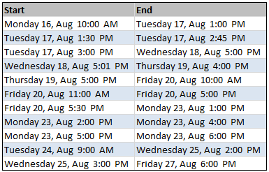
Also, Johnny logged the time he spent for every million atoms using, well, excel. Like this:
Your homework:
Johnny needs your help to figure out how many hours he worked in total (as well as for each million). He is already tired hunting a missing electron in the basement alleys. So don’t tell him to count manually. He wants to have an excel formula that tells him how many hours he worked given a start and end date in cells A1 and A2 respectively. Remember,
- Johnny never works after 6pm or before 9am
- Johnny never works on weekends.
- Lets say Johnny doesnt take any lunch breaks (he has developed a taste for those higgs bosons sandwich with positron milk shake).
So I am gonna go ahead and ask you to complete this homework before the weekend. When you got the correct formula, come back here and post it in comments. Ummkay?
More excel homework:
- Find out days overlapped between 2 dates
- Average of top 5 values
- More Home work | Formula tutorials & examples
PS: If you feel lost, that is because you have not seen office space. Go watch it.
PPS: if you still feel lost, that is because you do not know NETWORKDAYS. Go learn it.


44 Responses
Monday 23th 5 PM till Monday 23th 4 PM ? That is -1 hour for 1.000.000 atoms! Even better: Tuesday 17th 4 PM till 2 PM, -2 hours! I wish I could work like that 🙂
First, find out difference in Start / End Date, using Networkdays. So, in C2, type ‘=NETWORKDAYS(A2,B2)-1.
In D2, Find Start Time only, using ‘=TIME(HOUR(A2),MINUTE(A2),SECOND(A2))’
Repeat in E2 to Find End Time, ‘=TIME(HOUR(B2),MINUTE(B2),SECOND(B2))’
In F2, Calculate diff in Start / End Time ‘=E2-D2 ‘
Next, in G2, add Days from D3 to Time in G3 ‘=C2+F2
Finally, Express in terms of hours, and take off time between 6pm and 9am ‘=(G2*24)-(C2*15)’
I’ve changed a couple of the times given – cell A4 changed to 12pm, A6 to 6pm (doesn’t work at 7pm) and B10 changed to 6pm.
Total hours worked 86.5, average 7.86 hours per million.
Combining into one formula, looks a little like this:
=((NETWORKDAYS(A2,B2)-1)+(TIME(HOUR(B2),MINUTE(B2),SECOND(B2))-TIME(HOUR(A2),MINUTE(A2),SECOND(A2))))*24-(NETWORKDAYS(A2,B2)-1)*15
@Tessaes… sorry.. my bad. I guess I was too busy sympathizing with Johnny. I correct the image and data file. Try now 🙂
=SUM((NETWORKDAYS(A2,B2)-2)*TIME(9,0,0),TIME(18,0,0)-MOD(A2,1),MOD(B2,1)-TIME(9,0,0))*24
Whole days worked * hours in a working day + max possible hours to work from start to end of day + max possible hours to work from start of day to finish. Multiply by 24 to convert to hours.
Total time worked: 100 hours and 44 minutes
Hours per million (divide by 11): 9 hrs per million
D1 being 6pm
E1 being 9am
=(NETWORKDAYS(B3,C3)*($D$1-$E$1))-(TIME(HOUR(B3),MINUTE(B3),SECOND(B3))-TIME(HOUR($E$1),MINUTE($E$1),SECOND($E$1)))-(TIME(HOUR($D$1),MINUTE($D$1),SECOND($D$1))-TIME(HOUR(C3),MINUTE(C3),SECOND(C3)))
AVG: 7:31
SUM: 82:44 /3d 10h 44m
??
=(NETWORKDAYS(B3,C3)*($D$1-$E$1))
-(TIME(HOUR(B3),MINUTE(B3),SECOND(B3))
-TIME(HOUR($E$1),MINUTE($E$1),SECOND($E$1)))
-(TIME(HOUR($D$1),MINUTE($D$1),SECOND($D$1))
-TIME(HOUR(C3),MINUTE(C3),SECOND(C3)))
Rather than using:
TIME(HOUR(),MINUTE(),SECOND())
to convert time to integers and then back again to time, keep in mind that time in XL is simply stored as a decimal. You can save several steps by simply dropping the integer;
Either:
A2-INT(A2)
or
MOD(A2,1)
=SUM(C3:C13-INT(C3:C13)-(B3:B13-INT(B3:B13))+(NETWORKDAYS(B3:B13;C3:C13)-1)*9/24)
Ctrl+shift+enter gives 82 hours and 44 minutes where the 9 is the length of a workday.
I get 82.73 hours.
=(NETWORKDAYS(B3,C3)*9)- ((TIME(HOUR(B3),MINUTE(B3),SECOND(B3))-TIME(9,0,0))*24)- ((TIME(18,0,0)-TIME(HOUR(C3),MINUTE(C3),SECOND(C3)))*24)Whoops. Most people dont think of minutes as a decimal value.
Properly translated, I get 82 hours and 44 minutes.
If start and end dates are in cells B3 and C3 respectively, this formula calculates the hours he worked for the 1st million:
=24*SI(ENTERO(B3)=ENTERO(C3);C3-B3;C3-B3-ENTERO(C3)+ENTERO(B3)+9/24)+SI(DIAS.LAB(B3;C3)>2;(DIAS.LAB(B3;C3)-2)*9;0)
Hours Million
12,00 #1
01,25 #2
11,00 #3
07,98 #4
02,00 #5
06,00 #6
04,50 #7
02,00 #8
01,00 #9
14,00 #10
21,00 #11
Hours he worked in total: 82,73 hours (82 hours and 44 minutes)
Cleanest formula I can come up with is:
=((NETWORKDAYS(B3,C3)*(0.375))-(MOD(B3,1)-0.375)-(0.75-MOD(C3,1)))*24
This produces 82.73 hours (82:44) with Johnny being very efficient on the 23rd and completely slacking off on his last million weaseling his way to 21 hours–lets hope we aren’t paying him hourly. :o)
@ Michael. That is a great formula. Nice way to think in reverse of backing out hours from max hours. That’s neat.
Thank you, Abbas, much appreciated!
In my last message I wrote a Spanish formula. Now my English formula:
=24*IF(INT(B3)=INT(C3);C3-B3;C3-B3-INT(C3)+INT(B3)+9/24)+IF(NETWORKDAYS(B3;C3)>2;NETWORKDAYS(B3;C3)-2)*9;0)
Explanation for each million:
– If start and end dates are equal, subtract them: 24*(C3-B3)
– If start and end dates are not equal, the difference in hours is obtained and added a working day of 9 hours: 24*(C3-B3-INT(C3)+INT(B3)+9/24)
– For each number of days greater than 2 is added one more working day of 9 hours: NETWORKDAYS(B3;C3)-2)*9
Total hours: 82,73 hours
Just I changed my formula to include comma separated arguments:
=24*IF(INT(B3)=INT(C3),C3-B3,C3-B3-INT(C3)+INT(B3)+9/24)+IF(NETWORKDAYS(B3,C3)>2,NETWORKDAYS(B3,C3)-2)*9,0)
I hope not to have to reach one million messages!
this formula should work for any start date (in cell B3) and end date (in cell C3), and account for any amount of weekends between the start and end dates, to give you decimal hours taken for each million
=((24*(C3-B3)-(((NETWORKDAYS(B3,C3))-1)*15))-(IF((C3-B3)>=7,((FLOOR(((C3-B3)/7),1)+1)*48),0)))
where the multiplier 15 (just before the IF) is the number of hours between 6pm today and 9am tomorrow … if the work hours change, then this 15 would change accordingly
if the difference between the start and end dates is >= 7, then a non-working weekend is involved and you have to subtract 48 hours for each weekend … the FLOOR part is used to count how many weekends are involved and multiply accordingly
—Woody
The problem of writing formulas without testing them is to forget some parenthesis. My formula without known errors:
=24*IF(INT(B3)=INT(C3),C3-B3,C3-B3-INT(C3)+INT(B3)+9/24)+IF(NETWORKDAYS(B3,C3)>2,(NETWORKDAYS(B3,C3)-2)*9,0)
Another way to do the same:
=IF(INT(B3)=INT(C3),C3-B3,MOD(C3,1)-MOD(B3,1)+9/24+IF(NETWORKDAYS(B3,C3)>2,(NETWORKDAYS(B3,C3)-2)*9/24,0))*24
Total: 82.73 hours = 82:44. Always the same result!
As Abbas said, the Michael’s formula is great but can be simplified:
=9*(NETWORKDAYS(B3,C3)-1)+24*(MOD(C3,1)-MOD(B3,1))
Johnny always has worked 82.73 hours.
99 hours and 45 minutes.
Pedro, that is a brilliant formula.
@ Pedro – I agree with Michael, the formula is truly a great find.
I used networkdays + days360 to solve the problem of calcullating through the weekend
the catch is to put the parenthesis in the right place
(C3-B3)*24-((NETWORKDAYS(B3,C3)-1)*15+(DAYS360(B3,C3)-(NETWORKDAYS(B3,C3)-1))*24)
157.73 hours..!
The real atom splitter is..
http://www.cpearson.com/excel/DateTimeWS.htm
OOPS..! It’d be 77.73 hrs..!
Suppose I propose to get the result in column D. I will first format the column so that it has the format as DATE and type as HH:MM:SS.
Once the above is done simply get the difference of D column – C column in D.
Once you have copied the formula for all rows. Take the total of column D you will get the Total Hours as ;-> 250:44:00
correction to my earlier posting … criteria to see if a weekend is involved was wrong.
=((24*(C3-B3)-(((NETWORKDAYS(B3,C3))-1)*15))-(IF((WEEKDAY(C3)-WEEKDAY(B3))<0,((FLOOR(((C3-B3)/7),1)+1)*48),0)))
And, the formula is..
=If(And(Int(StartDt)=Int(EndDt),Not(IsNA(Match(Int(StartDt),
0,0)))),0,If(Int(StartDt)=INT(EndDt),
0+Round(24*(EndDt-StartDt),2),
(Max(Networkdays(StartDt+1,EndDt-1,0),0)+
Int(24*(((EndDt-INT(EndDt))-(StartDt-Int(StartDt)))+
0.375)/9))*8+Mod(Round(((24*(EndDt-Int(EndDt)))-9)+
(18-(24*(StartDt-INT(StartDt)))),2),
9)))
May atom splitting look easier now!
Chandoo, Let me validate my answer.
Is 77.73 hrs correct..?
Thank you everyone for such varied, elegant and awesome solutions. I found the ones by Michael and Pedro pretty clever. But there are so many other good formulas too.
I have prepared a solution workbook to show you how this works, You can download it here:
http://img.chandoo.org/hw/working-hours-between-2-dates-data-solution.xls
I will be doing a subsequent post next week explaining how you should attack this problem.
Thank you once again.. 🙂
@ Michael. Out-of-box thinking..! Quite nice!
@Chandoo, here is my explanation at your working hours between two dates explanation:
Total hours worked
=9*networkdays(start_date,end_date)-24*(start_time-9/24)-24*(18/24-end_time)
It is the Michel’s Formula – Longer Formula:
=networkdays(start_date,end_date)*9-24*(start_time-9/24+18/24-end_time)
=networkdays(start_date,end_date)*9-24*start_time+(9-18)-24*end_time
=networkdays(start_date,end_date)*9-9-24*(start_time-end_time)
Simplifying it is Pedro’s Formula – Shorter Formula:
=9*(networkdays(start_date,end_date)-1)-24*(start_time-end_time)
Explanation of last formula where:
n = networkdays(start_date,end_date)-1
If start_date = end_date Then
=24*(end_time-start_time)
End If
If start_date + n = end_date Then
=9*n+24*(end_time-start_time)
End If
In these formulas are 2 cases:
If end_time >= start_time Then
The positive difference in hours is added to 9*n.
End If
If end_time < start_time Then
The difference in hours is subtracted from 9*n.
End If
No one seemed surprised at the use of the mod… so I must be missing something big!
Is the mod used here to gather the decimal parts of the number?
I am struggling with the equation, most probably because the mod part escapes me altogether.
Thanks for all those pretty complicated questions that look so simple.
Hi Pedro and Chandoo,
I have tried both your formulas and unfortunately it does not give me the right information that I need…Here is my data and the formula that I have used for them. Here is what I need…
Work timings are : 06:30 AM till 18:30 PM from Mon – Fri
Working hours are 12 hours which is from 06:30 AM till 18:30 PM
Weekends are off, and holidays are off.
AO13 (Start Date) : 2/7/14 15:44 PM; AP13 (End Date) : 2/10/14 7:16 AM
Formula used: =(NETWORKDAYS(AO13,AP13)*12) – ((TIME(HOUR(AO13),MINUTE(AO13),SECOND(AO13))-TIME(6,30,0))*24) – ((TIME(18,30,0)-TIME(HOUR(AP13),MINUTE(AP13),SECOND(AP13)))*24)
This gives me the answer as 3.53 which is incorrect. The correct hours worked is 3:31:49
What am I missing from your formula ?
Hi Rajesh,
The result 3.53 hours is the same as 3 hours and 56 hundredths of hour. As you want is not the decimal format but the hour format.
3.53 hours = 3 hour + 31 minutes + 48 seconds.
Try this in a cell: = 3.53 / 24
And format as “Hour”
Pedro,
Thanks. I also realized that after I posted the comment; I tried various options and what I did then was to change the format of the cell to [h]:mm:ss to display the hours which are more than 24 hours. That solved the issue. And you are correct, this formatting that you suggested also did the trick.
Thanks for sending your comments. Really appreciate it.
Rajesh
can you please help me in getting the correct time difrence between….. incident opened date and time is 18/8/2014 8:21 am – closing time and date 20/8/2014 9:22pm working hours are 8: 30 am to 5 :00 pm for my office
I have a few discrepancy’s which I require assistance with to understand – i’m trying to work out how long a tech took to respond to a ticket
I have the following scenario’s
startdate 12/10/2015 23:33 end date 14/10/2015 07:30
using formula:
incorrect: -0.0478 Isn’t it?
=8*(NETWORKDAYS(C5,D5)-1)-24*((MOD(C5,1)-MOD(D5,1)))
@Lynette
Simply use
=End date Cell – Start date Cell
then format the cell as [h]:mm
By using this, it doesn’t take into account hours worked between 8:00 and 16:20 – nor does it remove weekends
I know the time doesn’t fall in working hours – but it still need to calculate the time it took in working hours counted together to advise how long it took before responding
IFS(AND(DAYS(C3,B3)=0,TIME(HOUR(B3),MINUTE(B3),0)>=TIME(9,0,0),TIME(HOUR(C3),MINUTE(C3),0)=TIME(9,0,0),TIME(HOUR(C3),MINUTE(C3),0)>=TIME(18,0,0)),(TIME(18,0,0)-TIME(HOUR(B3),MINUTE(B3),0))*24,
AND(DAYS(C3,B3)=0,TIME(HOUR(B3),MINUTE(B3),0)=TIME(18,0,0)),(TIME(18,0,0)-TIME(9,0,0))*24,
AND(DAYS(C3,B3)=0,TIME(HOUR(B3),MINUTE(B3),0)<TIME(9,0,0),TIME(HOUR(C3),MINUTE(C3),0)=TIME(9,0,0),TIME(HOUR(B3),MINUTE(B3),0)=TIME(9,0,0),TIME(HOUR(C3),MINUTE(C3),0)1,TIME(HOUR(B3),MINUTE(B3),0)>=TIME(9,0,0),TIME(HOUR(B3),MINUTE(B3),0)=TIME(9,0,0),TIME(HOUR(C3),MINUTE(C3),0)<=TIME(18,0,0)),(((TIME(18,0,0)-TIME(HOUR(B3),MINUTE(B3),0))+(TIME(HOUR(C3),MINUTE(C3),0)-TIME(9,0,0)))*24+(((DAYS(C3,B3))-1)*9)),
AND((WEEKDAY(C3)-WEEKDAY(B3))<1,(WEEKDAY(B3)+1)7,(WEEKDAY(C3)-1)1,TIME(HOUR(B3),MINUTE(B3),0)>=TIME(9,0,0),TIME(HOUR(B3),MINUTE(B3),0)=TIME(9,0,0),TIME(HOUR(C3),MINUTE(C3),0)<=TIME(18,0,0)),(((TIME(18,0,0)-TIME(HOUR(B3),MINUTE(B3),0))+(TIME(HOUR(C3),MINUTE(C3),0)-TIME(9,0,0)))*24+((7-WEEKDAY(B3)-1))*9+((WEEKDAY(B3)-2))*9))