

Last time I posted something on a weekend was almost a few years ago. I am making a rare exception to share a joyous news with all of you.
We bought our first car yesterday. It is a Maruti Suzuki Alto (link). See the picture below:
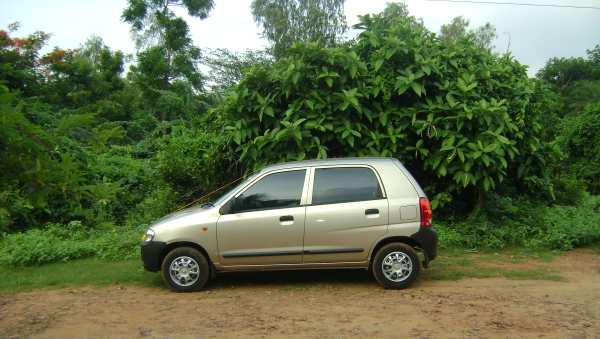
Ever since we became parents in September last year, the question of car was in our minds. There is no way we can bike with all 4. But few things bothered me,
- We are against loans and we wanted to buy our car on all cash.
- Since I started my own company, spending cash on car seemed dangerous.
- We wanted a car that serves our basic needs, nothing too fancy.
That was back in September 2009. Since then, we have been saving for a car. Thanks to Excel School, Project Management Templates, By June 2nd week, we have accumulated enough buffer to purchase a car.
Then we looked around for models and makes. Suddenly everything became a blur. But thankfully we didn’t get lost. We choose a very basic model made by one of the largest car manufacturers in the world – Maruti Suzuki. The model, Alto, seemed to be everywhere on roads. We went ahead and booked it last week. We got it home yesterday.
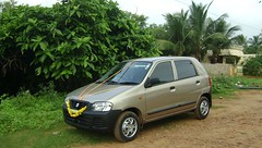 Few more specifics about the car,
- It can seat 4 people comfortably, 5 not so.
- The gears are manual, but the steering is power.
- It has A/C and a music system.
- We paid INR 3,40,000 (roughly US $7,300) for it, all on cash, no loan 🙂
- And of course, I don’t know how to drive!!!
Thank you:
Thank you so much for supporting me and my business all along. You inspire me everyday to be a better person and better businessman.
And of course, I should thank Excel too. It has changed me life.
Now, go have a good weekend, I need to figure out how to change from neutral to first gear without having the engine die.
PS: People who have been reading me since 2008 would point that this is indeed not my first car. Well, it is sort of, the camry was bought in US and sold.


29 Responses
Oh you had a camry? lol I need to go and read that post. Hope it works well for the family. God bless you man, and God bless that car. Pray over it and ask God to protect the car, you and your family. And I’m sure you’ll figure out the gears soon.
Many-Many Congratulations! Have a happy and safe drive. Always.
And since you have come to India after a long time, I advise you to refrain from ‘road rage’.
Congrats Sir!!!!
Congrats on your momentous experience! While I know the culture in the US is different from yours in India, I know the feeling you’re experiencing well. My wife and I have 5 incredible children and we are in the process of building a house that finally and truly will fit us all comfortably. I can totally empathize with the joy you and your family must feel with the new freedom a car brings you!
Chandoo, I can relate. For years BC (Before Children) we did everything with our bicycles, including the big weekend shop. With children, things tend to be a bit more complex if you want to move the whole family cum picnic hamper and nappy bags and toys.
Now, in New Zealand, everybody seems to have at least two cars per family member (slight exaggeration). We still do lots of things with the bicycle, but for some jobs, our little Honda Jazz is just right.
Good luck, and be easy on the cyclists!!
cheers, teylyn
Many Many Congratulations !! You bought absolutely right car !! Go for long drive and share your experience 🙂
Just found your Blog on Excel and had to say thankyou for helping us all out. Congrats on getting your first car. Must have been a special moment 😉
Congratulations Chandoo
I hope you and the family have many safe journeys and great experiances
Although I must say I am disappointed you didn’t by a Hyundai Excel ?
Congratulations !!!
The perfect car for India.
You don’t know how to drive – that should not be a problem – no one does on our roads but we do fine don’t we.!!
Congratulations Chandoo !! it is indeed a great joy to to be a car owner, and I think that it is the same all over the world. You made a good choice – the Suzuki Alto is a good reliable workhorse. Careful driving now….. B-)
Marvelous. How inspiring, and funny that someone who is an absolute genius at Excel does not know how to drive. There is hope for me yet in Excel. 🙂
Congratulations Chandoo,
Well earned..well deserved
Best regards,
Winston
Congrats Chandoo – all the best and enjoy your new car.
You bring joy to the world of excel!
Congratulations Chandoo, I dont know you, but i feel really happy for you. Im from Argentina, and I know how hard is to buy a car. Best regards from La Rioja, Argentina.
Pablo Molina.
Congrats !!
Hearty Congratulations Chandoo!
Your blog has helped me a lot in Excel and my daily work.
Wish you a safe and happy driving all along.
God bless all of you.
Thanks.
Congrats!
Now the only thing that’s missing is a bumpersticker.
“I keep track of my traffic violations with Excel”
/Loranga
@Stephen.. yes I did. It was a fun vehicle to ride. We had loads of fun and lots of long drives on it, thanks to amazingly simple US driving culture and ever so wide roads.
@Kapil… Road rage ?!? My wife actually blames me for driving too carefully 😛
@Saurabh… Thanks.
@Bryan… 5 kids?!! it must feel really exciting and tiring… happy parenting.
@Telyn…I used to bike while working in Copenhagen, Denmark. It is an excellent place to bike. Now we are in Vizag which is more of a hilly place. Riding a bike is an almost tedious experience here (also the air is quite polluted). Anyhow, I promise to go easy on cyclists. I will knock only one of them every week 😛
@Ayush and Saman… Thank you 🙂
@Hui.. there is a car named Excel?!? Alas, they dont sell it in India…
@Paresh: thanks. hehe, I think the danger is that even if you drive well, others on the road may not follow rules and thus can create problems for you.
@Pete… Thanks.
@Sabrina: Thank you. I must point out that I know driving. It is just that I have experience only in US where the steering is on other side and almost no cars have stick shifts.
@Winston, Shree, Nivedita, Vijay: Thank you so much.
@Paul.. Thank you Paul. While it is ridiculously easy and reasonably cheap to get a car in US, for rest of the world, purchasing a car is big thing, more so in developing countries like India. I am enjoying the vehicle so far.
@Loranga: Good bumper sticker. Except, I might run out of the row limit pretty soon.
Congratulations on your new car. Alto is a damn good car (I too own the same specs as your car).
http://en.wikipedia.org/wiki/Hyundai_Excel
Congratulations Mate !!! I know the glitters of buying first car !!! All the best Chandoo.
Congrats on the purchase.
Now all you need to do is fit mags and lower the suspension, install a turbo,add a couple of sub woofers for the rear and fit a spoiler kit (for more down force at the new high speeds you will achieve) and your ready to go….oh and need the fluffy dice to hang around the mirror.
Congrats and well deserved my friend.
RP
Congratulations to you and your family!
I am glad that the business you love and dedicate so much effort to has shown this great reward. Enjoy the fruits of your labour.
Hearty congrats Chandoo! I’m a new entrant to your club, but I’ll enjoy continuing to be part of it in future. Incidentally I’m also getting my first car, Alto, in a couple of days. I am glad your hard work and dedication have helped you to reach this heights – both professionally & financially – and I’m really surprised that you admit it openly. All the best, from a professor who uses Excel extensively in management teaching, and yet learning a lot of shortcuts & other useful applications. Learning never stops!
Nice post, honestly!
tbheadsets.wordpress.com
Hi, Chandee!
As the proud owner of a Tesla, I heartily recommend setting your sights on the model 3, which is due out in volume next year. Yes, it’s a lot more expensive, but it fits all the other requirements you have to a “T.”
You are to be congratulated for your incredible work and accomplishments. I wish you all the very best in NZ. It should be great fun. Never been there, but the photos are spectacular and the lifestyle seems wonderful.
Cheers!
John