Use Copy & Paste to Preserve References to Tables [Quick Tip]

Share

Facebook
Twitter
LinkedIn

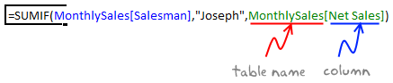
With Excel 2007, Microsoft has introduced a powerful and useful feature called as Tables. One of the advantages of Tables is that you can write legible formulas by using structural references. That means, you can write easy to understand formulas like this,

Structural references in Excel Tables - Example

[Help on SUMIF formula]

But, there is a problem. When you write these formula and drag the formula cell sideways to fill remaining cells, Excel changes table column references and thus makes your formulas almost useless.

Well, there is a simple workaround for this problem.

Use copy & paste.

Instead of dragging the cell to fill formulas, you can use copy & paste to fill the formulas. In this case, Excel will preserve all table references while changing the cell references accordingly. See this demo to understand:

Preserve Table References while Copying Formulas

Share your Table Tips & Tricks

Ever since I discovered the tables feature in Excel 2007, I have been using them to save time and simplify my work with data. Tables have several useful features that make life simple for analysts and data junkies everywhere.

What about you? Do you use Excel Tables? What are your top table tricks? Please share using comments.

More on Excel Tables

If you are using Excel 2007 or above, I encourage you to learn Excel Tables. They will make your life simpler. Go thru below articles to learn more,

Facebook
Twitter
LinkedIn

Share this tip with your colleagues

Excel and Power BI tips - Chandoo.org Newsletter

Get FREE Excel + Power BI Tips

Simple, fun and useful emails, once per week.

Learn & be awesome.

Welcome to Chandoo.org

Thank you so much for visiting. My aim is to make you awesome in Excel & Power BI. I do this by sharing videos, tips, examples and downloads on this website. There are more than 1,000 pages with all things Excel, Power BI, Dashboards & VBA here. Go ahead and spend few minutes to be AWESOME.

Read my storyFREE Excel tips book

Overall I learned a lot and I thought you did a great job of explaining how to do things. This will definitely elevate my reporting in the future.
Rebekah S
Reporting Analyst
Excel formula list - 100+ examples and howto guide for you

From simple to complex, there is a formula for every occasion. Check out the list now.

Calendars, invoices, trackers and much more. All free, fun and fantastic.

Advanced Pivot Table tricks

Power Query, Data model, DAX, Filters, Slicers, Conditional formats and beautiful charts. It's all here.

Still on fence about Power BI? In this getting started guide, learn what is Power BI, how to get it and how to create your first report from scratch.

13 Responses to “Convert fractional Excel time to hours & minutes [Quick tip]”

  1. Debraj Roy says:

    Hi Purna..

    Again a great tip.. Its a great way to convert Fractional Time..
    By the way.. Excel has two great and rarely used formula..

    =DOLLARFR(7.8,60) and =DOLLARDE(7.48,60)

    basically US Account person uses those to convert some currency denomination.. and we can use it to convert Year(i.e 3.11 Year = 3 year 11 month) and Week(6.5 week = 6 week 5 days), in the same manner...

  2. Jason says:

    This doesn't work for me. When applying the custom format of [h]:mm to 7.8 I get 187:12

    Any ideas why?

    • Hui... says:

      @Jason
      7.8 in Excel talk means 7.8 days
      =7.8*24
      =187.2 Hrs
      =187 Hrs 12 Mins

      If you follow Chandoo's instructions you will see that he divides the 7.8 by 24 to get it to a fraction of a day

      Simple, assuming the fractional time is in cell A1,

      Use below steps to convert it to hours & minutes:

      1. In the target cell, write =A1/24
      2. Select the target cell and press CTRL+1 to format it (you can also right click and select format cells)
      3. Select Custom from “Number” tab and enter the code [h]:mm
      4. Done!

  3. WhoKnows says:

    Hi, sorry to point this out but Column C Header is misspelt 'Hours Palyed'

  4. abhishek malik says:

    good one

  5. Julia says:

    So how do I go the other way and get hours and minutes to fractional time?

    • Chandoo says:

      If you have 7.5 in cell A1,

      - Use int(A1) to get the hours.
      - Use mod(A1,1)*60 to get minutes.

      If you have 7:30 (formatted as time) in A1

      - Use hours(a1) to get hours
      - Use minutes(a1) to get minutes.

      • Paula says:

        I had the same issue. You can solve it by changing the format as described above:

        Right click cell > Format Cells > (In Number tab) > Custom > Then enter the code [h]:mm
        ([hh]:mm and [hhh]:mm are nice too if you want to show leading zeros)

        • Jack Scarce says:

          Thanks guys, these are the tips I'm looking for.
          ...dividing the number of minutes elapsed by the percent change is my task - "int" is the key this time

  6. Srikanth says:

    It doesnt work for greater than 24 hours
    It returns 1:30 for 25.5 hours. It should have returned 25:30

    Ideally I would right function as
    =QUOTIENT(A1,1)&":"&MOD(A1,1)*60

    • Paula says:

      Sorry, replied to wrong comment....

      ----
      I had the same issue. You can solve it by changing the format as described above:

      Right click cell > Format Cells > (In Number tab) > Custom > Then enter the code [h]:mm
      ([hh]:mm and [hhh]:mm are nice too if you want to show leading zeros)

  7. Daniel says:

    Clever use of MOD here to extract the decimal part of a number. Divide a number containing a decimal by 1 and return the remainder. Humm. Very clever.

  8. Tomer says:

    Thanks very much, extremely useful !

Leave a Reply