fbpx
Search
Close this search box.

Calculate Payment Schedule [Homework]

Share

Facebook
Twitter
LinkedIn

While I was away, Hui did a splendid job of starting a new series called Formula Forensics. The idea is to break down formulas for difficult real-world problems so that we can understand them better.

In that spirit, I am giving you an interesting and tough formula homework.

Situation:

Imagine you work for Large Fries Inc. as a sales person. You sell fries, chips, curls and other coronary clog causing consumables. It is not a pleasant job, but you do it nevertheless. The economy is not good and you don’t want the paycheck to vanish!

The Large Fries Inc., much like any company large, has some crazy policies. One such thing is their payment policy for sales persons. It has 2 important rules.

  • You must earn at least $200 before they pay you.
  • There should be a gap of at least 7 days between successive payments.

Shown below is your sales data since October 1st. First column is date, second is your commission earned.
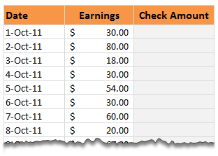
Calculate Payment Schedule in Excel - Homework

(enlarge to see all data)

Your Homework:

Your mission, if you choose to accept, is not really dangerous or explosive. Nevertheless, it is fun and challenging.

Write a formula in third column such that it show the amount of commission to be paid subject to the 2 conditions above. You can use a helper column if you want.

The downloadable file contains correct answers for you to verify your solution.

Download Workbook with Data

Click here to download the homework problem workbook. You can see the correct answers too (no formulas, just answer).

Go ahead and Solve

Go ahead and solve this and post your answers. I am really curious to know how you would solve this. Please share your explanations in the comments.

Some help & more

Facebook
Twitter
LinkedIn

Share this tip with your colleagues

Excel and Power BI tips - Chandoo.org Newsletter

Get FREE Excel + Power BI Tips

Simple, fun and useful emails, once per week.

Learn & be awesome.

Welcome to Chandoo.org

Thank you so much for visiting. My aim is to make you awesome in Excel & Power BI. I do this by sharing videos, tips, examples and downloads on this website. There are more than 1,000 pages with all things Excel, Power BI, Dashboards & VBA here. Go ahead and spend few minutes to be AWESOME.

Read my storyFREE Excel tips book

Overall I learned a lot and I thought you did a great job of explaining how to do things. This will definitely elevate my reporting in the future.
Rebekah S
Reporting Analyst
Excel formula list - 100+ examples and howto guide for you

From simple to complex, there is a formula for every occasion. Check out the list now.

Calendars, invoices, trackers and much more. All free, fun and fantastic.

Advanced Pivot Table tricks

Power Query, Data model, DAX, Filters, Slicers, Conditional formats and beautiful charts. It's all here.

Still on fence about Power BI? In this getting started guide, learn what is Power BI, how to get it and how to create your first report from scratch.

55 Responses to “Calculate Payment Schedule [Homework]”

  1. Stef@n says:

    Hey Chandoo
    please provide also a version for Excel 2003 !
    Regards Stef@n

  2. Will Clark says:

    Start by seeing the difference between the total earned and the total paid. Then see if there are six preceeding days of zero paid. (Added error checking when you start with less than 7 rows above).

    Fixed version:
    =IF(SUM(C$6:C6)-SUM(D$5:D5)>200, IF(ISERROR(COUNTIF(OFFSET(D6,-6,0,6,1),0)),0, IF(COUNTIF(OFFSET(D6,-6,0,6,1),0)>=6, SUM(C$6:C6)-SUM(D$5:D5),0)),0)

    Flexible version (you can change the parameters on the right):
    =IF(SUM(C$6:C6)-SUM(D$5:D5)>$G$23, IF(ISERROR(COUNTIF(OFFSET(D6,-($G$24-1),0, ($G$24-1),1),0)),0, IF(COUNTIF(OFFSET(D6,-($G$24-1),0, ($G$24-1),1),0)>=($G$24-1), SUM(C$6:C6)-SUM(D$5:D5),0)),0)

  3. Will Clark says:

    Note: The display isn't wrapping the long formulas... It's all there, just need to copy-and-paste the whole thing, or go here: http://pastebin.com/PbMTHmp1

  4. jason says:

    ....this place makes you work 7 days a week!?!

    3rd condition perhaps?

  5. Fred says:

    @Jason. Sales can come in everyday of the week, such as a supermarket. I don't necessarily look at it as a person but a sales entity.

    That said, there is a flaw in the exercise. Looks like this sales person/entity is getting paid in arrear. In reality you don't really know what the commission is a day later or 2 days later or even 3 days later.

  6. Shelby says:

    Hi Chandoo,

    Does your excel school teach you how to understand complex formulas like Will Clark's?

  7. PrasadDN says:

    Hi Chandoo..

    D6 should have =IF(AND(G6>=7,(SUM($C$6:C6)-F6)>200),SUM($C$6:C6)-F6,"")

    Helper columns
    F6 should have =IF(ISNUMBER(D5),(D5+F5),F5)
    G6 should have =IF(F6=F5,G5+1,1)

    I know this can be done without helper column also, but i prefer easy formula than complicating it myself 🙁

    F column keeps track of total earnings and G column keeps track of how many days since last pay check made.

    Regards,
    Prasad DN

  8. PrasadDN says:

    Like Will, this can be made flexible by changing 7 and 200 in D6 with H24 and H23.

    Forgot to mention I have included 2nd helper column in G, so your instruction and limits go pushed to H column. 🙂

  9. NukeRiskGuy says:

    I named the limit cell 'Limit_Min' and I started my formula in D7 instead of D6 to make it cleaner (actually, I toyed with using a helper column to create a string value for the summing ranges and using INDIRECT in my formula to get rid of error checking, but it would be harder to understand):

    =IF(ROW()-6>=6,IF(AND(SUM($C$6:$C7)-SUM($D$6:$D6)>=Limit_Min,COUNTIF($D1:$D6,">0")=0),SUM($C$6:$C7)-SUM($D$6:$D6),0),0)

    It's not pretty, but it works

  10. NukeRiskGuy says:

    Here it is with a line break in the middle:

    =IF(ROW()-6=6,IF(AND(SUM($C$6:$C7)-SUM($D$6:$D6)>=Limit_Min,
    COUNTIF($D1:$D6,">0")=0),SUM($C$6:$C7)-SUM($D$6:$D6),0),0)

  11. Daniela Munteanu says:

    Hi Chandoo,

    I've created a formula for D6 that uses a helper column E.
    The formula for D6 is =IF(SUM($D$5:D5)=0,IF(AND(SUM($C$5:C6)>=$H$23,(B6-$B$6)>=6),SUM($C$5:C6),""),IF(AND((SUM($C$6:C6)-SUM($D5:D$6))>=$H$23,(B6-INDEX($B$5:B6,MATCH(COUNTIF($D$5:D5,">0"),$E$5:E5,0)-1,1))>=6),SUM($C$6:C6)-SUM($D5:D$6),""))

    I separated the first payment from the other ones so i used the first if to do that. If no previous payments are find then the formula checks if the total earnings until that day are at least 200 and if the difference between the curent date and the first entrace of the table is at least 6.

    For the case when I have previous payments, the formula checks if the difference between the total earnings until that day and the total payments made until that day is at least 200 and if the difference between the curent day and the date of the previous payment is at least 6. To find the date of the previous payment i used index, with the help of the E column.

    The helper column has this formula: =IF(D6>0,COUNTIF($D$6:D6,">0")). I've used this helper column to count the number of payments.

  12. Kyle McGhee says:

    Not the first method that came to mind but I wanted to challenge myself:
    =IF(D5=$D$5,"",IF(( AND( SUM( INDEX($C$6:$C$46, IFERROR( MATCH( 1E+30,$D5:D$6,1) +1,1), ):C6) >=$G$23,( B6-INDEX( $B$6:$B$46,IFERROR( MATCH( 1E+30,$D5:D$6,1)+1,1),) +1)>=$G$24)),SUM( INDEX( $C$6:$C$46,IFERROR( MATCH( 1E+30,$D5:D$6,1)+1,1),):C6),""))

    For this to work the non-payment days need to be "" rather than 0, otherwise MATCH(1E+30,$D5:D$6,1) will pull in zero if it is the last number in the lookup range.
    I am using IFERROR(MATCH(1E+30,$D5:D$6,1)+1,1) to find the last number above the active cell; if there is no match, a payment has yet to be made, so 1 is used (first cell in index range). This is used as the starting point of both the "number of days" check and the” >= $200 check ranges”. If it passes both checks, then the same sum formula is used to calculate the payment.
    The IF(D5=$D$5,"",…) is used to prevent a circular reference in the first row of the schedule. If the prior cell equals the column header then it is the first cell in the range and can therefore be safely excluded since 7 days cannot have yet passed.
    This also allows for non-contiguous dates as it subtracts the dates to find the number of days, rather than assuming every row is +1 day.

  13. Kyle McGhee says:

    As with Will above, the formula is not being displayed properly. Let me see if this works:
    =IF(D5=$D$5,"",
    IF((AND(SUM(INDEX($C$6:$C$46,
    IFERROR(MATCH(1E+30,$D5:D$6,1)+1,1),):C6)>=$G$23,
    (B6-INDEX($B$6:$B$46,
    IFERROR(MATCH(1E+30,$D5:D$6,1)+1,1),)+1)>=$G$24)),
    SUM(INDEX($C$6:$C$46,
    IFERROR(MATCH(1E+30,$D5:D$6,1)+1,1),):C6),""))

    If not, just copy and paste the comment into word or notepad and take the formula from there

  14. Prem Sivakanthan says:

    What great fun..!!! Here is my solution: I’ve used the words ‘smallerthan’ and ‘greaterthan’ in my formulas rather than the symbols, as last time I tried to use those symbols in a post, it did some very strange things. No helper columns used. Before we get stuck into the solution, I used two named formulas: rw= IF(ROW()smallerthan12, ROW()-1,11)
    ct=INDEX('payment schedule homework'!$D$6:$D$46, ROW()-rw):'payment schedule homework'!$D5. These two formulas are used to create dynamic arrays, which are fed to the countif formula below, to ensure there is a gap of at least 7 days between payments.

    The formula that is at the crux of this solution is as follows:
    =(SUM($C$6:$C6)-SUM($D$5:$D5)greaterthan200)*(SUM($C$6:$C6)-SUM($D$5:$D5))*(COUNTIF(ct, "=0")greaterthan5)

    Here is a breakdown, CSI-Chandoo style:
    The first part of the formula (SUM($C$6:$C6)-SUM($D$5:$D5)greaterthan200), is testing to see if the sum of all payments (up to the current row, which is the current date) minus the payments made to date, is greater than 200; and if it is true, then it is multiplying true (read 1) by this difference. Note where the $ signs are in the formula. The second part of the formula (COUNTIF(ct, "=0")greaterthan5) is testing to ensure there have been no payments made in the last 7 days.

    The above solution uses Boolean logic instead of the IF formula to make decisions on what calculation to do…something that often comes in handy when you don’t want to have a million nested if’s.

  15. Andy Holaday says:

    I have nothing to add in the way of formulae. I dinked around and found myself in hopelessly circular methods. Kudos to those who posted solutions!

    What I did notice using the solutions of others is this is probably not a good incentive model for commissions. Why? A good follow-up exercise for those wondering would be to apply the techniques Hui posted on this site for Monte Carlo simulations:

    http://chandoo.org/wp/2010/05/06/data-tables-monte-carlo-simulations-in-excel-a-comprehensive-guide

    What you find out is the expected payout is pretty much equal, regardless of the dollar and date thresholds.

    It's understood though, this was meant to be a logic challenge, not a real business model.

  16. sam says:

    Define cTot = SUM(C$6:C6)-SUM(E$5:E5)
    Define pInt = ROW()-MAX(($E$5:E5>0)*ROW($E$5:E5))

    Formula in E6 that can be dragged down

    =(cTot>=200)*(pInt>6)*cTot

  17. Phil says:

    Interesting to see other ways of doing this. Here is my version. Its a bit long, but works.
    First it checks to see if the sum of sales since the last payment was made total more than $200 :-

    SUM(OFFSET(C6,-(ROW(C6)-MAX(IF($D$5:D5"",ROW($D$5:D5)+1)))),0):OFFSET(C6,0,0))>=200

    and that the last payment was at least 7 days ago :-

    ROW(C6)-(MAX(IF($D$5:D5"",ROW($D$5:D5)))))>=7

    When all true, it uses the offset function to sum column C from the day after the last payment to current day :-

    SUM(OFFSET(C6,-(ROW(C6)-(MAX(IF($D$5:D5"",ROW($D$5:D5)+1)))),0):OFFSET(C6,0,0))

    The formula in total :-
    =IF(AND(SUM(OFFSET(C6,-(ROW(C6)-(MAX(IF($D$5:D5"",ROW($D$5:D5)+1)))),0):OFFSET(C6,0,0))>=200,(ROW(C6)-(MAX(IF($D$5:D5"",ROW($D$5:D5)))))>=7),SUM(OFFSET(C6,-(ROW(C6)-(MAX(IF($D$5:D5"",ROW($D$5:D5)+1)))),0):OFFSET(C6,0,0)),"")

  18. Phil says:

    Forgot to add, it is an array formula {....}

  19. Peter Vousden says:

    Hi,

    Never posted on here before so here goes as I was interested by the puzzle set.

    My version of the non-helper column solution is:

    "=IF((B6-$B$6)=200,(B6-$B$6)>=6),SUM($C$6:C6),0),IF(AND(ROW()-LOOKUP(2,1/(($D5:D$60)*ISNUMBER($D5:D$6)),ROW($D5:D$6))>=7,SUM(C6:INDIRECT("C"&LOOKUP(2,1/(($D5:D$60)*ISNUMBER($D5:D$6)),ROW($D5:D$6))+1))>=200),SUM(C6:INDIRECT("C"&LOOKUP(2,1/(($D5:D$60)*ISNUMBER($D5:D$6)),ROW($D5:D$6))+1)),0))"

    To explain the thought behind it:

    1) The first IF statement simple looks for the first entries and counts for the number of entries and the total to be greater than the constraints and enters '0' if they are not yet met or the total once they are met.

    2) The second IF statement then covers entries after one valid entry has already been made - $302 on the 7th. It then again checks for the number of days since that entry by finding the row value of the last non-zero value and also the total earnings from that point.

    ROW()-LOOKUP(2,1/(($D$6:D50)*ISNUMBER($D$6:D5)),ROW($D$6:D5)) - calculates the number of days since the last payment by current row minus row of last payment.

    SUM(C6:INDIRECT("C"&LOOKUP(2,1/(($D5:D$60)*ISNUMBER($D5:D$6)),ROW($D5:D$6))+1))>=200),SUM(C6:INDIRECT("C"&LOOKUP(2,1/(($D5:D$60)*ISNUMBER($D5:D$6)),ROW($D5:D$6))+1) - adds up the earnings in column C from the row after the last payment to the current row via an indirect reference.

    3) If this is yet to match the constraints it enters '0' otherwise the value of the outstanding earnings payment.

    Comments welcomed!

  20. VaraK says:

    My solution:
    I left check amount on Oct 1 as blank. and the below formula starting from Oct 2. In my worksheet this goes in D10 cell: =IF(AND((SUM($C$9:C10)-SUM($D$9:D9))>199,COUNTBLANK(D4:D9)=6),SUM($C$9:C10)-SUM($D$9:D9),"")

  21. Peter Vousden says:

    Not too sure why the posting process has added additional zeros...? As in '(($D5:D$60)*'. Please note that this should be "(($D5:D$6)*".

  22. Matt S says:

    in order to solve this one, I pulled out the datedif formula:

    =IF(AND(DATEDIF($B$6,B7,"d")+1/COUNT($D$4:D6)>=7,SUM($C$6:C7)-SUM($D$6:D6)>199),SUM($C$6:C7)-SUM($D$6:D6),"")

  23. Here is my solution using only one formula:
    '=IFERROR(AND(SUM(OFFSET(C6,0,0,-(MOD(ROW()-7,7)+1))) >= 200,MOD(ROW()-7,7)+1 >=6,F5=0) * SUM(OFFSET(C6,0,0,-(MOD(ROW()-7,7)+2))),0)'

  24. Correction, you must place this into the C column: =IFERROR(AND(SUM(OFFSET(C6,0,0,-(MOD(ROW()-7,7)+1))) >= 200,MOD(ROW()-7,7)+1 >=6,D5=0) * SUM(OFFSET(C6,0,0,-(MOD(ROW()-7,7)+2))),0)

  25. Correction, the above works if you place the formula into the F column. For the D, "Check Column, you will use this formula: =IFERROR(AND(SUM(OFFSET(C6,0,0,-(MOD(ROW()-7,7)+1))) >= 200,MOD(ROW()-7,7)+1 >=6,D5=0) * SUM(OFFSET(C6,0,0,-(MOD(ROW()-7,7)+2))),0)

    Just note that the formula checks if the cell above it is zero ("D5=0"), so it doesn't matter where you put it, you will just have to make sure the formula correctly points to cell above it.

  26. Jon says:

    `=IF(AND((SUM($C$6:C6)-SUM($D$5:D5))>$G$23,IF(ROW()>11,COUNTIF(OFFSET(D6,-6,0,6),0)=6,0)),SUM($C$6:C6)-SUM($D$5:D5),0)`

    This is what I came up with.

  27. Jon says:

    =IF(
    AND(
    (SUM($C$6:C6)-SUM($D$5:D5))>$G$23,
    IF(ROW()>11,
    COUNTIF(OFFSET(D6,-6,0,6),0)=6,
    0)),
    SUM($C$6:C6)-SUM($D$5:D5),
    0)

    First time posting code to this website, I'll split it up.

  28. Jon says:

    Looks like many of my solutions are very similar to others. Pretty straight forward.

  29. =IF(SUM(C$6:C6)-SUM(D$5:D5)>199, IF(ISERROR(COUNTIF(OFFSET(D6,-6,0,6,1),0)),0, IF(COUNTIF(OFFSET(D6,-6,0,6,1),0)>5, SUM(C$6:C6)-SUM(D$5:D5),0)),0)

  30. Daffy333 says:

    My answer was a lot like Prem's, but without the named range. Before I added the formula, I added 3 new rows below row 4, so that the "over seven days" references wouldn't refer above row 1, if you get my meaning. I then added the following:

    =--(SUM($C$8:C9)-SUM($D$8:D8)>$G$26-0.01)*--(COUNTIF(D3:D8,"=0")+1>=$G$27)*(SUM($C$8:C9)-SUM($D$8:D8))

    A couple double unaries (sounds like a Dr. Suess title).

    Thank you for the challenge!

  31. Chris Byham says:

    I wanted to push myself and use an array formula to complete this, so here goes:

    In cell D6, the formula is {=IF(ROW(C6)-MAX(($D$1:D5>0)*(ROW($D$1:D5)))>=$G$24,IF(SUM(C6:INDIRECT("C" & MAX(($D$1:D5>0)*(ROW($D$1:D5)))+1))>=$G$23,SUM(C6:INDIRECT("C" & MAX(($D$1:D5>0)*(ROW($D$1:D5)))+1)),0),0)} (holding CTRL+SHFT + ENTER)

    ROW(C6) returns the current row number.

    The array formula MAX(($D$1:D5>0)*(ROW($D$1:D5))) gives the highest 'non-zero' row position across the range, so looks from the top of the column down to the cell immediately above the current and returns the latest payment row. G24 contains the payment frequency, so has to be 7 or more days since the last payment.

    The array formula SUM(C6:INDIRECT("C" & MAX(($D$1:D5>0)*(ROW($D$1:D5)))+1)) sums the earnings from the current row back up to the row immediately below the last payment row. The rest is a simple If formula to check the payment amount in cell G23 has been reached.

    A great challenge - thanks once again Chandoo!!

  32. Richard Kehl says:

    I liked sam's approach. But what if there were mising dates.
    So I keyed off the dates.

    Define pInt or as pInt3 =$B6-MAX($B$6:$B6*($D$5:$D5>0))+1

    Define cTot = SUM(C$6:C6)-SUM(D$5:D5) --sam's, except I used Check Amount column
    Define pInt = ROW()-MAX(($D$5:D5>0)*ROW($D$5:D5)) --sam's, except I used Check Amount column

    Formula in D6 that can be dragged down --sam's, except I used Check Amount column
    =(cTot>=200)*(pInt3>6)*cTot --sam's, except I used Check Amount column

    Thanks sam - I was having hard time until I saw your approach

    Also I defined pInt2 = DATEDIF(MAX($B$6:$B6*($D$5:$D5>0),$B6,"d")+1
    works the same as pInt3

  33. [...]  Their most recent challenge tempted me so much that I had to try it. [...]

  34. Ante says:

    I just read this part of web so I am posting my solution late.

    Formula has tu be copied at cell D12 (no payouts for first six dates) and than copied down.
    =IF(SUM(D6:D11)>0;0;IF((SUM($C$6:C12)-SUM($D$6:D11))>199;(SUM($C$6:C12)-SUM($D$6:D11));0))

  35. Jijo Titus says:

    Hi Chandoo,

    After Long long hours of experimenting with formula finally got a solution. please someone review and let me know if there is any mistake so that i can improve this formula.

    **Formula pasted in column F**
    =IF(AND(SUM($C$4:C4)>=200,COUNT($B$4:B4)=7),SUM($C$4:C4),IF(AND(SUM($C$4:C4)-SUM($F$3:F3)>=200,COUNT($B$4:B4)-(COUNTIF($F$3:F3,">=200")*7)>=7),SUM($C$4:C4)-SUM($F$3:F3),"-"))

  36. Jijo Titus says:

    Regarding my previous post....**I have not used any helper column for this

  37. Jijo Titus says:

    hey chandoo...went through my formula again but this is not working...(not able to identity the 7 day limit) apologies please remove my post 🙁 ..am a beginner and not able to understand the above posts

  38. Ketan Sharma says:

    Hi Chandoo,

    Please provide a solution for this. I find solutions offered here quite complex.

    Thanks 

  39. Robert says:

    It appears that no matter what the first 6 days will be $0.  Assuming you can not have the formula in the first 6 rows (perhaps that is not fair, but what scenario would this be a problem in?), this formula will work if entered in D12.

    =IF(SUM(D6:D11)>0,0,IF((SUM($C$6:C12)-SUM($D$6:D11))>$G$23,(SUM($C$6:C12)-SUM($D$6:D11)),0))

  40. [...] Unul din blogurile de excel la care sunt abonata este http://chandoo.org/wp si aseara am primit newsletter cu noua postare de pe acest blog. In aceasta postare cititorii erau provocati sa creeze formula pentru calcularea programului de plata a unui reprezentant de vanzari. (Calculate Payment Schedule Homework) [...]

  41. Vijaykumar Shetye says:

    Enter the following formula in cell D12 and drag down the same.

    =IF(COUNTIF(D6:D11,">0"),0,IF(SUM(C$6:C12)-SUM(D$6:D11)>=200,SUM(C$6:C12)-SUM(D$6:D11),0))

    Vijaykumar Shetye,
    Goa, India

  42. Pundalik Rathod says:

    Hey Guys... I am late to this forum but not least... here simple formulla for this tricky question...

    =IF(MOD(COUNT($B$2:B8),7)=0,SUM(B2:B8),"")

    Pundalik Rathod

  43. Alex M says:

    Here's my formula and I quite proud of the fact that I was able to do it in one formula 😀

    '=IF(AND(SUM($C$6:C6)-SUM($D$5:D5)>$G$23,(COUNTIF'
    '($D$5:D5,0)-COUNTIF($D$5:D5,">0")*($G$24-1))>='
    '($G$24-1)),SUM($C$6:C6)-SUM($D$5:D5),0)'

    I hope this formula shows up properly.

  44. Daniel says:

    Ok, here is my solution ^^

    =IF(AND((SUM($C$6:C7)-SUM($D$6:D6))>=$G$23,COUNTA($C$6:C7)>=((COUNT($D$6:D6)+1)*$G$24)),SUM($C$6:C7)-SUM($D$6:D6),"")

    Leaving c6 blank or with:

    =IF(SUM($C$6:C6)>=200,SUM($C$6:C6),"")

  45. Debbie says:

    It's amazing how many different solutions people have come up with!

    I have a helper column G with formula: =IF(D5>0,ROW(D6),G5)

    And here's the solution for column D:
    =IF(SUM(INDIRECT("C"&G6):INDIRECT("C"&ROW(D6)))>=200,IF(COUNTIF(INDIRECT("B"&G6):INDIRECT("B"&ROW(D6)),">0")>6,SUM(INDIRECT("C"&G6):INDIRECT("C"&ROW(D6))),0),0)

    Probably could have used an "AND" function instead of the extra "IF", but I forgot about it, and this does work.

  46. Alex says:

    Hey guys,
    I just started following chandoo and I'm learning a lot with all of your solutions, thanks a lot!
    My solution is rather simple:

    =IF(AND(WEEKDAY(B7,2)=5,SUM(C2:C7)>=$G$24),SUM(C2:C7),IF(AND(WEEKDAY(B7,2)=6,D6=0,SUM(C1:C7)>=$G$24),SUM(C1:C7),0))

    It worked pretty well.

    All the best,
    Alex

    • Alex says:

      Breaking down:

      =IF(AND(WEEKDAY(B7,2)=5,SUM(C2:C7)>=$G$24),SUM(C2:C7),
      IF(AND(WEEKDAY(B7,2)=6,D6=0,SUM(C1:C7)>=$G$24),SUM(C1:C7),0))

  47. cnestg8r says:

    Sam's elegant solution can be enhanced by the simple addition of two more definitions, e.g.,

    =(cTot>=MinUSD)*(pInt>(MinDays-1))*cTot

  48. Faizan says:

    Hi,
    I tried with this formula and it is working fine (based on salary is paid exactly after 7 days IE 8th day only accumulating 200$).

    =IF(AND(WEEKDAY(B7)=7, SUM(C1:C7) > 200), "Payment Due " & SUM(C1:C7), IF(AND(WEEKDAY(B7) = 1, ISBLANK(E7)), SUM(C1:C7)))

    Regards,

    Faizan

  49. ELIENAY JUNIOR says:

    I tested most of the formulas here, and none worked as expected from the example that chandoo gave in the spreadsheet. I haven't tested all the formulas in the comments yet, because I would spend hours doing this. I tried to solve this challenge and I couldn't and look, I have an advanced level, 3 years of study left. So far I haven't seen any logic to solve this type of problem and nothing makes sense to me, this displacement of lines takes away anybody's patience! I ask Chandoo to post the spreadsheet with the formula, as I believe this is possible with VBA

Leave a Reply