
 We have a macbook at home (we have a name for it too, we call it Shimla, the most romantic place for us). Like all latest macbooks, this one too came with a trail version of iWork. Even though I have used iWork before, this time I wanted to compare iWork numbers with Excel. In this post, I want to highlight 7 really cool features for iWork and how Microsoft excel can benefit from implementing the same.
1. iWork comes with sexy templates
When you try to make a new Numbers document, iWork asks you to select from some of the templates. The templates are really practical and very cool. For eg. they have a template for creating a check-list, product comparison worksheet, household budget. These are really easy to use and work to the point.
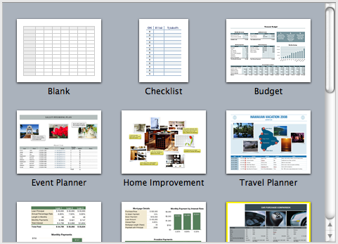
With excel 2007, MS introduced several new templates and gave us an option to import templates from web. But still, users resort to quite a few workarounds when it comes to building a neat looking worksheet. We all could benefit if something like this is available in Excel.
2. Simple but effective Paste Options
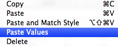
When you copy some values in to clipboard and try to paste them, iWork gives you an option to “paste values” and “paste and match styles”. 2 most commonly used paste options.
In excel, this is usually hidden in paste special menu (in 2007, paste values is available as a menu choice as well). Excel veterans know the ALT+ESV shortcut by heart. It would be cool to have these options highlighted in the menus and given easy to remember shortcuts.
3. Making Checkboxes, Sliders, Steppers ad List boxes is very easy
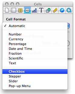
In iWork Numbers, to get a checkbox in a cell, all you need to do is format the cell as “checkbox”. You can also format a cell as slider, stepper or “pop-up menu” (usually known as combo box).
This is very easy compared to all the form control based stuff we are used to Excel. If MS implements this idea, we dont need to resort to sneaky tricks to get a bunch of checkboxes in excel or use wingdings font.
4. Quick summary of data

Whenever you select a bunch of numbers, iWork Numbers displays 5 quick statistics about the data, in the status area of the numbers application. (Unlike excel, iWork numbers has status bar in the left side).
Excel also shows the quick summary in the status bar, but usually the sum of values. (In excel 2007, you can configure the stats you want to see, thus mimicking this behavior. But it would surely help if these 5 stats are “always on” by default.
5. Cleaner Menu / toolbar area

While MS is going towards ribbon based interfaces for all their applications, iWork keeps the UI relatively simple and uncluttered. The toolbar area, shown below contains the vital buttons to make a filter, format a cell, create a chart, insert a function, table and change views. Everything else is buried one level deep.
This could be a more effective way to expose a complex application’s functionality. MS should consider these UI options as well.
6. Inspector Dialog for all the formatting options

Excel has a ton of dialogs to format cells, charts, drawings, printer settings, tables and more. In iWork, there is one dialog for all of these, called as inspector window. Using this you can setup printer options, page layout, table design, cell formatting, chart formatting, font, text, paragraph settings, drawing shape formats and other inserted object (such as movies) formats. Based on the selected item, the inspector window shows the corresponding tab where you can adjust the formatting.
This could be a great way to reduce the popup fatigue in Excel. In Excel 2007, MS introduced new popups that further complicated the way even a simple chart axis formatting. We all could benefit if MS implements simpler dialog boxes modeled after the inspector.
7. Switch rows and columns in charts intuitively
In iWork Numbers, to switch rows and columns in a chart, all you had to do is select the chart and then click on the little button that appears next to data range of the chart.


In excel you can do this using “select data” options of the chart. But doing this without leaving the worksheet is much more intuitive and cooler.
Have you tried iWork Numbers?
Apple is famous for its design sense and beautiful products. iWork is no exception. It is a visual treat to work with iWork.
What is your opinion about it?


12 Responses
You can also group values by a categorical column, and then do aggregation (sum, average, etc.) for each group. That is really useful when doing your taxes, etc. I haven’t tried using those aggregates for a chart, but if that works, that would also let you create histograms.
Numbers has a more semantic approach to spreadsheets: it’s not just a huge table where every cell is the same. You can have header rows and columns (that get ignored in formulas) and separate, independent tables on the same sheet.
It really all comes down to market share. Microsoft owns the corporate world with Excel and that alone will take some major change to undo. As long as they keep up with other software, MS Office will continue to dominate on a large scale. Also, major companies tend to have MS operating systems and not MAC.
It will be interesting to see if this changes as the younger generation ages.
Nice comparison Chandoo!
Great idea to show the other side!
Few days ago I saw this software and that was very impressive.
The main difference (for me) is the areas within the sheet where I can set different widhts for the columns (for example budget template).
I tried to export the templates to xls format and chech how these looks like in excel. The formating lost or modified, the areas went to separate worksheets.
But anyway Numbers is intuitive, simple, esthetic. Love at first sight.
Hey Guys, Has anyone seen this problem? Excel cannot complete task with available resourses. Choose less data or close other applications. I have down loaded Hotfix and SPC3 and still have the problem. I currently have a workbook with with 65 spreads sheets that link, macro’s etc… about 6.74MB. Have not had this problem before. I also tried to go to C:\documents and settingg/username\application data\microsoft/excel. I get to documnets ansd settings, but don’t see application data\microsoft\excel.
Can you help?
It’s made my day to find there’s a keyboard shortcut for Paste-Special-Value! You say “Excel veterans know the ALT+ESV shortcut by heart” —- but what’s the ESV bit mean ?!?!
D’oh!
I must follow the links – to where all is explained.
I must follow the links – to where all is explained.
I must follow the links – to where all is explained.
I must follow the links – to where all is explained.
Yes, there are some very nice features in Numbers that I’d like to see in Excel. Yet Numbers is a far inferior product. There are so many tasks that I can easily do in Excel, that I find very difficult to manage in Numbers. For example, simply adding cell borders, takes at least three clicks (or more) in Numbers and it’s not a very intuitive process. Also, formatting cell values is a complete nightmare. And yes the menu bar is cleaner, but is just because they put everything you need in that silly Inspector dialog box. The Ribbon may not be great, but it is much easier to find and perform the tasks I need than using the Numbers Inspector Box, which also, by the way, always seems to hover in the wrong place. Frankly, Numbers is a pedestrian product when compared to Excel. Which is disappointing because I have had a Mac as my home computer for over 20 years and I’m still waiting for a spreadsheet program that isn’t from MS.
This answer is for Alasdair about the shortcut for Paste Special:
ESV means that you press hold Alt, then you press E, then S and finally V 😉
Personally, I like iWork Numbers more than Excel. But at the company I work for, they still use Excel (as we all know MS dominates the market) and don’t have any policy to give a try to iWork Numbers. It’s pity.
The real advantages of Numbers:
– blank canvas on which you can place several, independent tables
– much higher graphic capabilities that allow users to create stunning business reports, impossible to create with Excel.
Yes, Numbers is not as powerful as Excel, not even close; but it’s only at version 2. Give it a few years.
Hi,
I need some help here…
I am using excel 2007 for pc, color-based filtering, date filtering ( ability to recognize dates and categorize them as months) are the major functions I use on the tables I create.
I wonder if i can get it done by iwork numbers… I want to switch to mac but advanced sorting and filtering capabilities are crucial for my work. from what I have seen numbers do not seem to get this accomplished.
for example i have sales records for each row, each row contains information regarding customer name, invoice number, date, amount, then i highlight the unpaid amount cells in yellow, and i can sort based on color so i see all unpaid invoices… i also type open orders in red font, i can also sort that by color, so instantly i can see open orders…
can you please comment whether this can be done in numbers?
thank you
Have a look at the Create and Edit Tables vids half way down
http://www.apple.com/iwork/numbers/