
JSON (JaveScript Object Notation) is a popular and easy format to store, share and distribute data. It is often used by websites, APIs and streaming (real-time) systems. But it is also cumbersome and hard to use for performing typical data tasks like summarizing, pivoting, filtering or visualizing. That is why you may want to convert JSON to Excel format. In this article let me explain the process.
1. Why Convert JSON to Excel?
Excel is a more familiar and easy to work with format for your data. Also, when setup properly Excel files (such as CSV or XLSX or XLSB) take up less space than their JSON counter parts. More importantly, performing data tasks like calculating formulas, creating pivots or making charts would be easier with Excel format as against JSON.
Overview of This Guide
In this guide, we’ll walk through multiple methods to convert JSON to Excel, including manual methods using Excel’s built-in tools, automated methods using Python, and third-party online tools. Whether you’re working with small or large datasets, there’s a solution for you. Let’s dive in and explore how you can make this transformation efficiently.
2. Understanding JSON Format
Before jumping into the process of converting JSON to Excel, it’s important to understand JSON format. JSON is a lightweight data format that’s easy for both us and computers to read and write. It’s primarily used to transmit data between a server and a web application, often in APIs or data feeds.
What Does JSON Look Like?
At its core, JSON is a collection of key-value pairs that are organized in objects and arrays. JSON data can be quite flexible, allowing it to represent both simple and complex data structures. It supports various types of data, including strings, numbers, booleans, arrays, and objects.
Let’s consider the following example of JSON data representing information about a few employees in a company:
{
  "employees": [
    {
      "id": 1,
      "first_name": "John",
      "last_name": "Doe",
      "email": "johndoe@awesomechoc.com",
      "position": "Chocolatier",
      "hire_date": "2023-06-15",
      "skills": ["Baking", "Cocoa Sculpting", "Confectionary"]
    },
    {
      "id": 2,
      "first_name": "Jane",
      "last_name": "Smith",
      "email": "janesmith@awesomechoc.com",
      "position": "Marketer",
      "hire_date": "2024-02-20",
      "skills": ["Packaging", "Product Design", "Field Sales"]
    },
    {
      "id": 3,
      "first_name": "Emily",
      "last_name": "Johnson",
      "email": "emilyj@awesomechoc.com",
      "position": "Accountant",
      "hire_date": "2024-08-30",
      "skills": ["XERO", "Excel", "AR / AP consolidation"]
    }
  ]
}
Breaking Down the JSON Example
- Objects and Arrays:
- The main JSON data structure in the example above is an object, denoted by curly braces
{}. - Inside this object, there is a key called
"employees", which maps to an array (denoted by square brackets[]). - The array (list) contains multiple objects, each representing a single employee.
- The main JSON data structure in the example above is an object, denoted by curly braces
- Key-Value Pairs:
- Inside each employee object, you’ll find several key-value pairs. For example,
"id": 1tells you the employee’s ID, and"first_name": "John"specifies the first name of the employee. - Some of the values in the JSON are simple data types (like strings or numbers), while others, such as the
skillskey, are arrays that hold multiple values.
- Inside each employee object, you’ll find several key-value pairs. For example,
- Nested Data:
- The
skillsfield is an example of nested data. It’s an array within the employee object, which further contains multiple string values representing different skills. This kind of nested data can be difficult to work with directly in Excel, which is why conversion and flattening are necessary.
- The
Challenges of Working with JSON in Excel
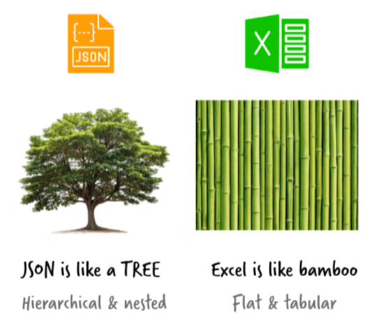
As you can see, JSON is hierarchical while Excel prefers data in a flattened, tabular format.
If you try to import JSON directly into Excel without transforming it, you might end up with a jumbled mess of data.
For example, in the above JSON, the "skills" field would result in a list being placed into a single cell if not properly flattened. Additionally, nested objects, like the employee object, would need to be expanded into separate columns (e.g., "id", "first_name", "last_name") for the data to be usable.
This is why it’s essential to convert JSON to Excel in a way that ensures all data is properly structured in rows and columns for analysis. Let’s explore some methods to accomplish that.
3. Methods for converting JSON to Excel format
There are many ways to convert JSON to Excel. My preferred technique is to use Power Query in Excel to convert the data quickly and elegantly. But you can also use other techniques. Let’s go thru each of these in detail.
JSON to Excel conversion (step by step):
What you need: You need a JSON file with your data. Download this sample data if you don’t have any.
- Go to Data > Get Data > From File > From JSON
- Select the JSON file on your computer (or on the network location)
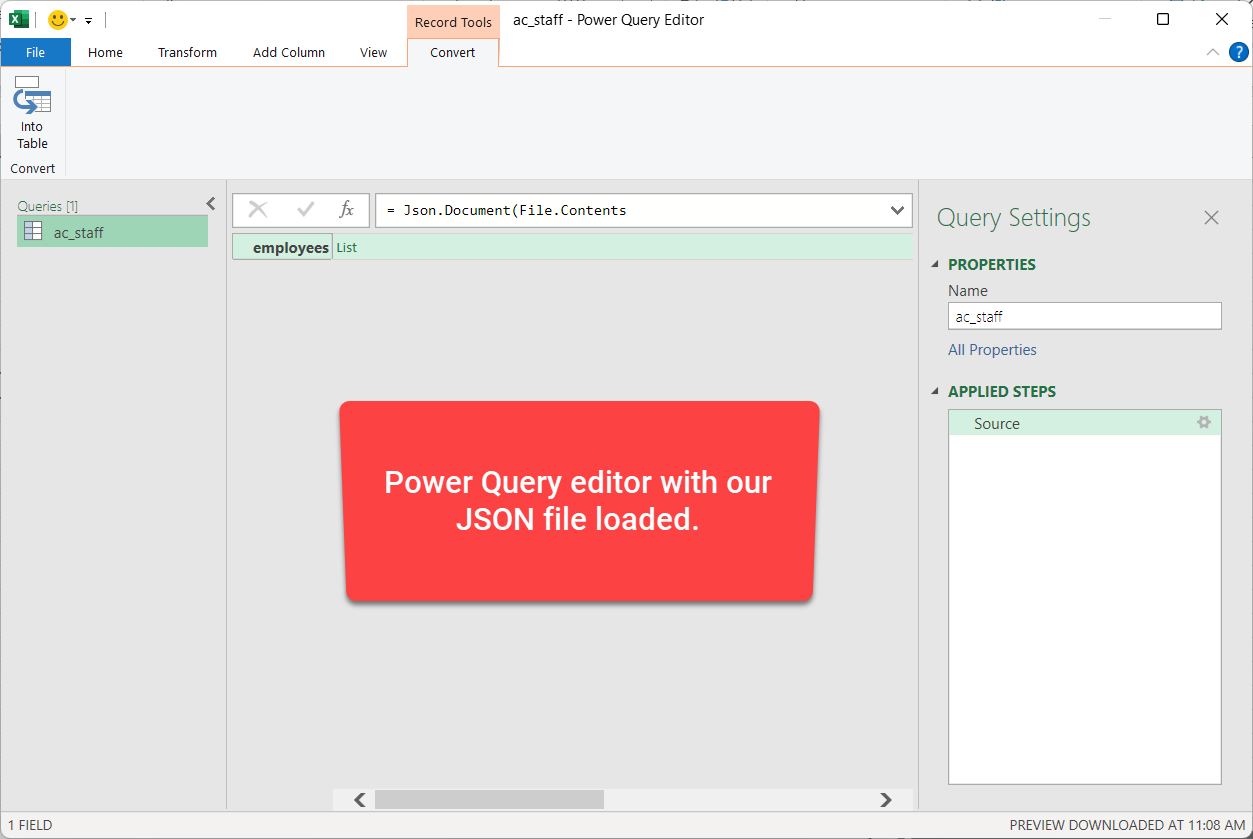
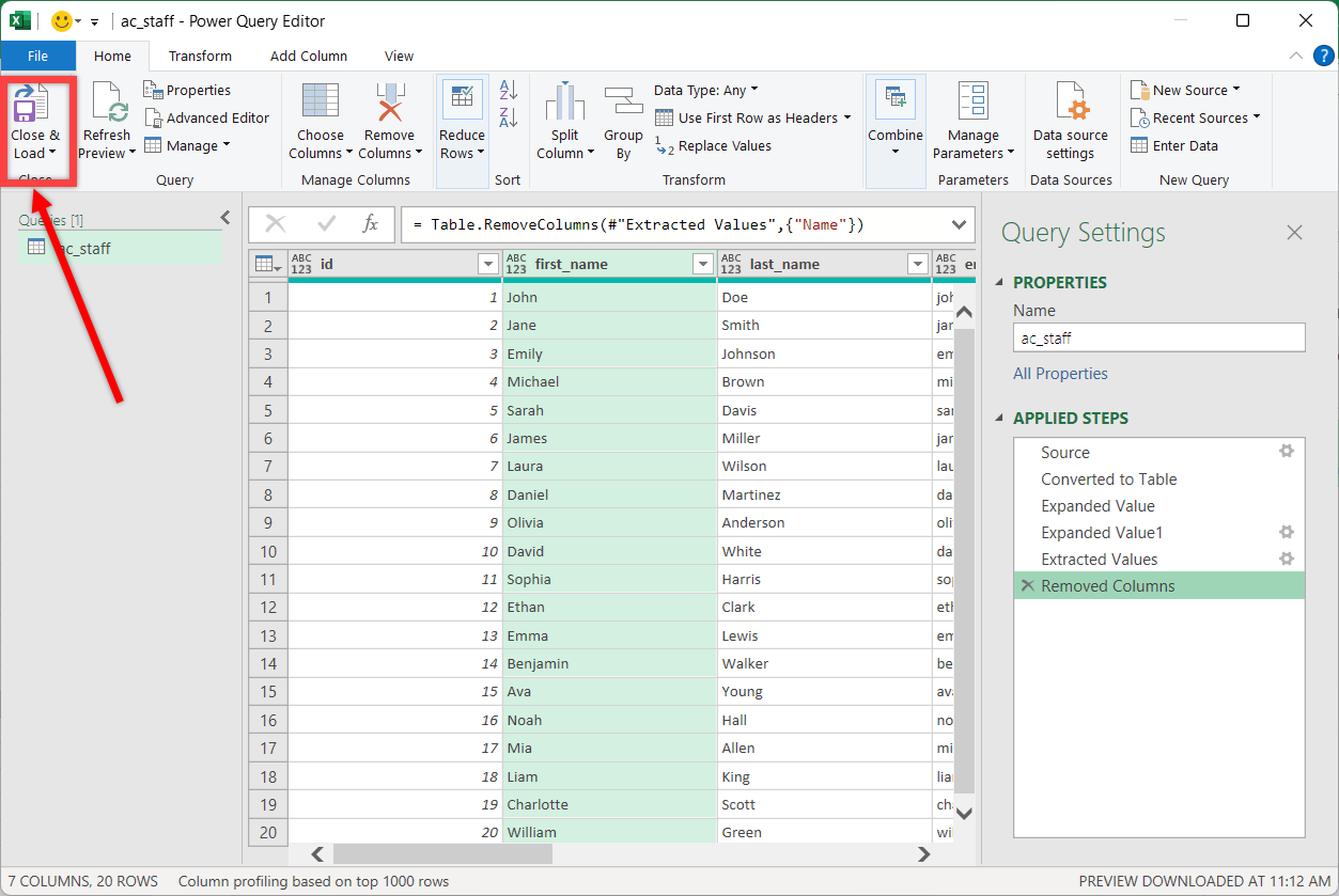
- This will open Power Query editor with your JSON file. Here is a snapshot of how that would look like:
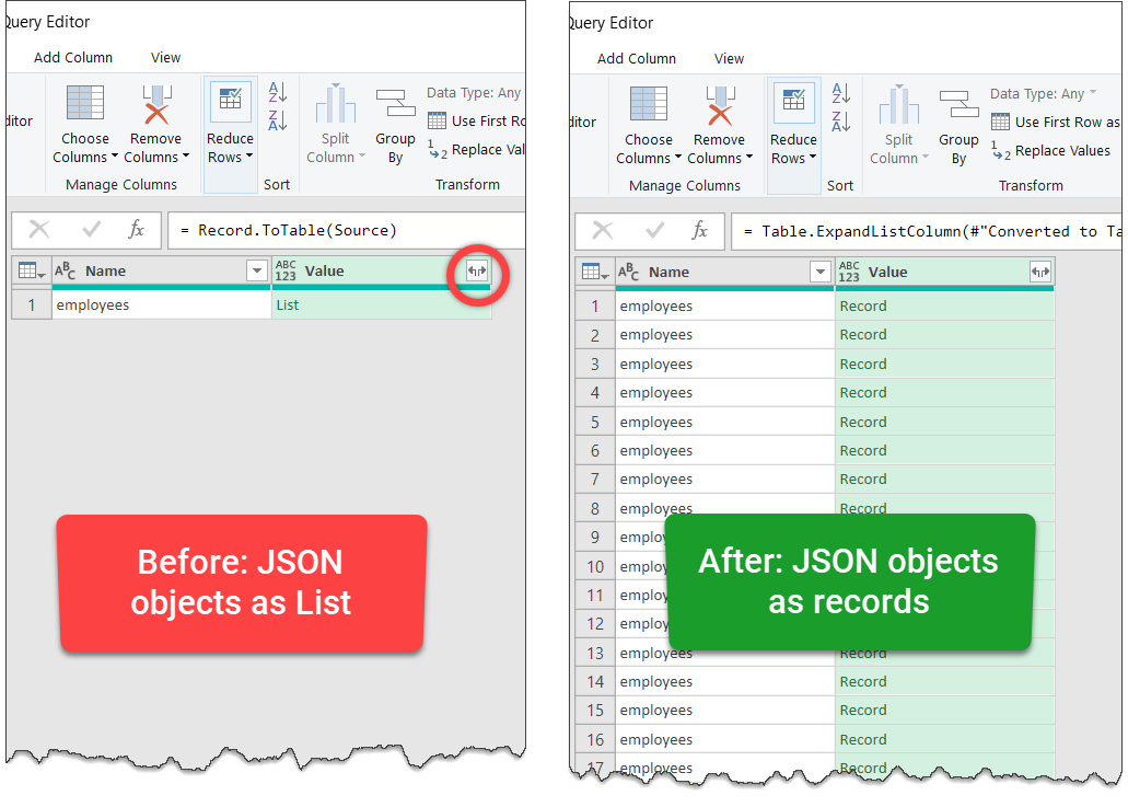
- Using the “convert” ribbon, convert the JSON listing to a “table”.
- Now you will have a “list” of all the JSON records (or objects). Click on the Expand button on the list column and select “expand to new rows”.
- This should show all the records of the JSON (see below)
- Expand the Value column again to see the contents of the records.
- If you have any “nested” or “hierarchical” data in your JSON, you must expand these columns again. But this time, use the “extract values…” option so you can see them all comma separated in the same column.
- Once you have all the necessary data in Power Query, remove any columns you no longer need by right clicking on them and selecting “remove” option.
- When ready, use the Home ribbon > Close & Load to bring the data to Excel.
Quick Demo of JSON to Excel conversion:
Here is a quick video demo of the process in Power Query.
Things to keep in mind when converting JSON to Excel with Power Query ??:
- Nested Data: If your JSON has nested data elements (for ex: skills attribute in our example above), you need to recursively expand all these items. But don’t expand them to “new rows” as this will create duplicate data. Instead just use “extract” option and get them all in one column with a delimiter like comma or semi-colon.
- Data type conversion: By default Power Query may convert your data to relevant data types. But always double check this and apply any conversion necessary.
- Preview vs. Load: Power Query Editor shows a preview of the JSON file for first 1000 rows, but actual conversion will only happen when you click on “close and load” button in Excel. So don’t freak out if you don’t see all the data in PQE (PQ Editor). It should appear when you load data to Excel.
- 1 Million Row Limitation: Excel spreadsheets can only hold 1,048,576 rows (just over 1 million). So if your JSON is really big, you need to think of another method. Here is an example of how to use Excel if you have more than 1 million rows of data.
Pros & Cons of using Excel to convert JSON:
Pros:
- Quick and easy: Power Query in Excel offers a quick, easy and straightforward way to convert JSON to Excel.
- FREE: Excel based conversion is free unlike paid methods.
- Refreshable: Should your JSON files change or update, you can quickly refresh the Power Query connection to see updated data in Excel. This means any reports or calculations you build on top of the JSON will automatically update, thus providing up to date information.
Cons:
- Hard to work with deeply nested data: If your JSON has multiple levels of nesting or hierarchies, then the Power Query based approach requires “drilling” to all these levels. As data can change often, if a new level of nesting appears in future, your Power Query refresh can fail.
- Requires understanding of Power Query: While PQ is not deeply technical, it is not easy either. So if you are not familiar with PQ, you will find this method hard to use. Here is an excellent beginner tutorial on Power Query with 4 powerful examples.
JSON to Excel conversion with Python (step by step):
Why Use Python for JSON to Excel Conversion?
While Excel’s Power Query can handle basic JSON imports, Python is often the better choice when dealing with large datasets, deeply nested JSON structures, or automating repetitive tasks. Using Python, we can efficiently read, manipulate, and export JSON data to an Excel file in just a few lines of code.
Installing Necessary Python Libraries
To begin, install the required libraries:
pip install pandas openpyxlThese libraries will help us process the JSON data and save it in an Excel-friendly format.
Loading JSON Data in Python
Consider the following employee data stored in JSON format (sample file).
{
  "employees": [
    {
      "id": 1,
      "first_name": "John",
      "last_name": "Doe",
      "email": "johndoe@awesomechoc.com",
      "position": "Chocolatier",
      "hire_date": "2023-06-15",
      "skills": ["Baking", "Cocoa Sculpting", "Confectionary"]
    },
    {
      "id": 2,
      "first_name": "Jane",
      "last_name": "Smith",
      "email": "janesmith@awesomechoc.com",
      "position": "Marketer",
      "hire_date": "2024-02-20",
      "skills": ["Packaging", "Product Design", "Field Sales"]
    }
  ]
}
We can load this JSON file into Python using:
import json
import pandas as pd

# Load JSON data from a file
with open("employees.json", "r") as file:
    data = json.load(file)
Converting JSON to a Pandas DataFrame
Since the JSON structure contains a list under the "employees" key, we extract and convert it to a DataFrame:
df = pd.DataFrame(data["employees"])This will transform the data into a tabular format, making it easier to analyze and manipulate.
Exporting Data to an Excel File
To save the structured data as an Excel file:
df.to_excel("employees.xlsx", index=False, engine='openpyxl')This creates an Excel file employees.xlsx, which can be opened in Excel for further processing.
Handling Nested JSON Data
If the skills field is stored as a list, Excel might not display it properly. We can flatten this field:
df["skills"] = df["skills"].apply(lambda x: ", ".join(x) if isinstance(x, list) else x)Now, each employee’s skills will be stored as a comma-separated string, making it easier to read.
Automating JSON to Excel Conversion
For repeated tasks, we can automate the conversion by scheduling this Python script to run daily or whenever a new JSON file is added.
Python provides a scalable and efficient way to process JSON data and export it to Excel, making it ideal for large datasets and automation needs.
Converting JSON to Excel with External Tools
If you don’t want to get your hands dirty with Power Query or Python based approaches, you can also use online tools to quickly convert JSON to Excel format.
1. Online JSON to Excel Converters
These web-based tools allow users to upload a JSON file and instantly download an Excel file:
- JSON to Excel by TableConvert
- Converts JSON to structured Excel tables.
- Allows previewing and editing before download.
- Supports additional formats like CSV and Markdown.
- JSONFormatter.org JSON to Excel
- Free tool with a simple drag-and-drop interface.
- Supports large JSON files.
- JSON to CSV
- Upload your JSON file and download the CSV
These tools are great for quick, one-time conversions, but they may have file size limitations and require manual steps each time.
2. Using Power BI to convert JSON to Excel
If you prefer to use a desktop software to convert JSON to Excel formats (like CSV or tables), you can use Power BI Desktop too. This doesn’t have 1 million row limitation so you ca use it to parse very large JSON files. The approach is same Excel Power Query technique, but the final data ends up in Power BI. You can either copy the table at the end of load process or use it directly inside Power BI to analyze the data.
Final Thoughts
If your JSON files are simple enough, just use Power Query in Excel to get the output the way you want. You can refresh this anytime your data changes.
On the other hand if your files are large or you need more control, use Python code samples above and tweak them to your needs.
If you have any questions, leave a comment so I can help you.


24 Responses
I’d suggest simply using the subtotal function and filtering the data using the Win/Loss column. You get the same results and the formula is more comprehensible.
@John
That is one option.
There are times however when you want to see the whole data table or a filtered subset and still want to produce summary reports against an unfiltered field.
Is there a particular reason why you are using a comma and the unary (–) operator for the second array in the SUMPRODUCT formula? It seems to work the same if you were to string the arrays together using the asterisk (*). The advantage is that SUMPRODUCT treats the entire string of arrays as a single array.
@Mathew
Your correct, There is no difference.
I thought it may have been easier to explain this method.
Is there a way to do this on a large set of data? As in ~100,000 rows? When I try I get an error because the formula becomes too long. It says the max length of a formula is 8,192 characters. Excel 2010.
How do I incorporate a specific text within a cell for the second array. For instance, – -(C7:C13=”Apple”)
when I chose a specific text the formula does not work.
@RB
I am not sure what is the issue as if I use the sample data in the post the following work fine
Count:
=SUMPRODUCT(SUBTOTAL(3,OFFSET(C7:C13,ROW(C7:C13)-MIN(ROW(C7:C13)),,1)), –(C7:C13=”L”))
Sum:
=SUMPRODUCT(SUBTOTAL(3,OFFSET(C7:C13,ROW(C7:C13)-MIN(ROW(C7:C13)),,1)),(C7:C13=”L”)*(D7:D13))
You may want to check that there are no leading or trailing spaces in your list of Apples
I should have given a better explanation. Heres my situation. I have a column with cells filled with names like Column 1, Column 2, Pier 1, Pier 2, etc. If the cell just contained Pier and searched for that it works. But because it has other characters in the cell its not recognizing the pier. So how can I extract specific characters of a string of text in this formula?
Hopefully this was a better explanation
Hello-
This formula works pretty well for me except that it slow down excel and prevents some of my macros from working. I was wondering if there was a way to program this in VBA so that excel isn’t always trying to recalculate it. I would like to use a push of a button to get it to run then paste in a cell.
Thanks!
I am trying to sum filtered data in a column, but would want to ignore the negative values in the column. How to go about doing this?
@Akshay
Why not just add a filter to that column to only show the values greater than zero?
The negative values are required for reporting purposes, but their effect on the total is distorting the required output. Please advise.
@Akshay
I’d suggest making a post in the Chandoo.org Forums
http://forum.chandoo.org/
Attach a sample file to simplify the task
I have this working for counting and summing, however, I have a list and for the second array, I need a criteria. That is, I’m looking for b13:b200=”01.??.??” or =left((a1,2) or something like that. These types of criteria matches do not appear to work as I get a blank as a result.
Thanks!
@Bob
As your formula b13:b200=”01.??.??” looks like you are trying to check the first day of the month of the range
What about trying Day(B13:B200)=1
Hai Experts,
i understood this formula well and working fine in MS Excel 2013
but when the same am trying to place in google Spreadsheet it shows error as
“SUMPRODUCT has mismatched range sizes. Expected row count: 1. column count: 1. Actual row count: 2014, column count: 1.” and as a result #VALUE! Appears in cell.
Can anyone please help me how would i get it done in Google Spread sheet
or is there any other formula as a substitute for this.
Thank you very much.
thanks for providing this.. but why does excel keeps on prompting Circular referencing in cell D3?
@Vivek
I don’t know
I just downloaded the file and it is working fine and not showing that error
Goto the Formulas, Calculation Options Tab and check that Calculation is set to Automatic
What version of Excel and Windows are you using ?
I know that this forum is for MS Excel, but I am trying to help someone who is working in Google Sheets. The below formula works in Excel but Google Sheets returns:
“SUMPRODUCT has mismatched range sizes. Expected row count: 1. column count: 1. Actual row count: 39000, column count: 1.” and as a result #VALUE! Appears in cell.
This is the same problem asked by Srichirin above. Does anyone know if there is a formula for Google Sheets that will replicate what MS Excel does?
=SUMPRODUCT(SUBTOTAL(3,OFFSET($C$6:$C$39500,ROW($C$6:$C$39500)-MIN(ROW($C$6:$C$39500)),,1)),- -($C$6:$C$39500=H1),($D$6:$D$39500))
Trying to find a SUMPRODUCT formula that counts the word Closed by date for the last 7 days in a filtered list.
=COUNTIF(M:M,”>”&TODAY()-7) works ok for unfiltered count Column M contains Closure dates (blank if open) and Column L is Status Open or Closed
@ Terry
Please ask the question at the Chandoo.org Forums
https://chandoo.org/forum/
Please attach a sample file to ensure a quicker more accurate answer
I used this formula and worked like a charm! But, now I’ve been requested to use it but adding not one but two criteria in the same formula. For instance the sum I was doing added negative and positive numbers. I’ve been asked to use the exact same formula but adding that only positive numbers were considered… any idea on how to do this?
How exactly do you do sum filtered cells when two criteria are need not just one?
Thank you so much brother literally I have been struggling since morning to get the sum of the filtered category, however, after reading your blog attentively i got my solution, so thanks a lot once again.