
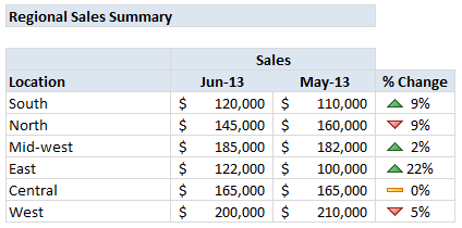
Pop quiz: What is wrong with below report?
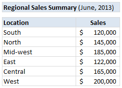
At first glance, it looks alright. But if you observe closely, you realize that it is not telling the entire story. Just looking at regional sales numbers, you have not much clue what is going on with them.
So how to improve it?
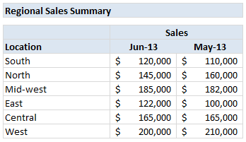
1. Add context
In order to know whether a number like $120,000 sales in South is good or bad, you need to provide some context. For example, if you include previous month sales figures, suddenly $120k is comparable to some other number. This tells a better story than a simple number alone.
You can also try these,
- Target values
- Same month last year values
- YTD, QTD values
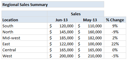
2. Add % Change
When you have 2 numbers like $120k and $110k in a report, anyone looking at them are going to mentally calculate the % change from last month to this month. This is easy for numbers like 120 and 110, but if your numbers are like 36,450 and 43,150 then calculating % change values will take time.
Why force your audience to do this mental math? Instead show these %s on the report.
3. Highlight bad numbers
Another way to enhance your report is to highlight poorly performing regions. Since each region is different, comparing sales of one with another is not good. But you can compare % change (from previous month / same month last year / targets etc.) and highlight poorly performing regions. This can be done with conditional formatting.
So lets go ahead and do it for our report above.
3.1 Add conditional formatting
Just select the %change column, go to conditional formatting > icon sets > and choose an arrow icon set that you fancy.
![]()
3.2 The default formatting kinda sucks
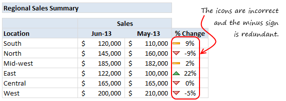
We are not done yet. If you look at the default icon formatting, it looks in-accurate. We are seeing red colored, down-ward arrows even when there is a positive change. And, when the % change is negative, we no longer need minus sign (-) because it will be indicated by down arrow.
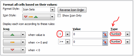
3.3 Fix the conditional formatting icons
Select the cells again, go to home > conditional formatting > manage rules. Select the rule and edit it (you can double click on the rule to edit).
Change the rule type as shown below.
3.4 Remove the minus sign
Select the %change column once again, go to format cells (ctrl+1) and set the custom formatting code 0%;0%
This will make sure that even when the percentage is negative, Excel will not show the sign (minus symbol).
Related: More on custom cell formatting in Excel.
So there you go. A regional sales report that tells better story.
Key ideas to keep in mind
In your reports, try to provide as much context as possible. This can be done by
- providing comparisons
- including additional statistics (sum, count, median etc.)
- indicating the time frame of the report
- highlighting bad numbers or areas that require attention
- giving user a choice to change report criteria (interactive features).
Do you follow these principles when making reports or dashboards?
I try to observe these ideas in all my dashboards. What about you? Are you using simple numbers in your dashboards?
Go ahead and tell us how you are making your dashboards better, in comments.
Analyze data and make reports / dashboards often?
If your job involves data analysis, reporting & dashboards, then you will love our Excel School program. In this online course, you will learn how to use Excel to analyze data with formulas & pivot tables, highlight important stuff, create stunning charts & tables, make them interactive and put everything together to weave an informative dashboard & more.
Please click here to know more about Excel School program and join us.


53 Responses
Clever trick with the arrow icons and suppressing the negative sign!
Excellent article, Chandoo, I love the way you present the topic with simple but irresistible ideas to improve the presentation of the reports. Keep up the great work!!
Yet again an absolutely brilliant article. Thanks Chandoo
As usual: another clear, informative and useful article. Thanks and keep up the blogging!
simple yet very effective and clearly communicated
THANK YOU!
Well communicated article…simple but effective!
Question – how did you re-align the icons? In your second picture they are not aligned to the left edge?
I have added an extra column (spacer) and adjusted the borders to get the effect.
Thanks
Love the tip!
Is there a way to align the arrows closer to the data as opposed to the left edge of the cell without using a spacer column?
Another technique is,
1. set up conditional formatting to show “icon only”.
2. Then in next column show the percentages
3. Now align the icon column to middle or right. This will move the icons.
Hi Chandoo, how are you ?
kya hum hindi me bat kar sak thay hai??
Excellent tips! Thank you!
The only thing I would add is to not forget TOTALS at the ends of columns or rows (as required). People tend to forget this often and it takes away the “big picture” information.
One thing i want to add is you can add top values and bottom values to grasp auditions eye in dashboard.
Nice! I would also recommend right-justifying the % Change column. It’s much easier to read numbers of varying digits if they’re right-justified.
Great article and love the humor:
“The default formatting kinda sucks”
Hope my laugh didn’t disturb the rest of my cubemates.
Learning can be fun!
Hi there, good article, but can you provide the file. I had the below issues
3.3 Fix the conditional formatting icons
after doing this the “-” remained but the arrows changed.
Also, 0% shows a green arrow, how do you make this orange arrow?
tks
It is a good idea to leave a margin of error in case of “no change” state – e.g. we would not want to to show a green arrow if the sales increased from $165,000 to $165,001. The simple way to do that is to adjust the values in step 3.3 to something like 0.001 and -0.001 instead of 0.
Thank you Krzysztof Sikora!! That done the trick.
I got a problem with the above – how can you setup the format so that it handles good/bad arrow direction when some cells in the column may on any given month be negatives or positives ? This sometimes is the case in expenses data.
Eg Actual -7 Budget -9 in the case of a transfer “credit” situation that should flag “red” as bad – you were expecting more back. But if the same cells then revert to costs of Actual 7 Budget 9 you have done “green” good. Is there a formula that can be used to correctly apply the right rule depending on whether the cells values are the scenario a or scenario b the right way?
Hi Cal,
There are a few different ways to accomplish this with a formula. It’s basically the same principle as having revenue and expenses in an income statement where a “good” result is:
Actual revenue is greater than budget
Actual expenses are less than budget
Add a column for your A/B scenario. Instead of A or B, use 1 or -1 in this column to flag each row. Flag rows with a -1 if the criteria is the same as your transfer credit scenario where the actual is less than the budget and this “good”. Then add another column that multiples your Variance (% Change) by your Scenario column.
This will inverse the sign for the rows where Actual < Budget = Good.
Alternatively, you can use an IF or CHOOSE function to create a statement that will do this. Then you could use the value (a,b) or (1,2) in your Scenario column.
Your final variance column can then be used for the source of the conditional formatting.
Let me know if this is not clear.
Thanks,
Jon
Gday Jon,
Thanks for coming back to me. I am stil a bit stuck. I think I will have to “phone a friend” as they say on the tv show “deal or no deal”
Cheers
C
I’d be happy to take a look at your file. You can find my email if you click on my name above. “email a friend”… 🙂
Great article! Kudos for the simple & clear presentation!
I love the idea of targets. One of the things I’ve been doing (by request) is looking at fractles using the =percent() formula.
For example, what does 90% of my data do relative to my target? This gives me a value I can assess relative to a target on a percentage basis.
My only hangup with Excel is that I also need the converse result on my arrays. (Insert group challenge here)
For example, if I have a target of 600 seconds 90% of the time, I need to know both the number of seconds at 90%, and the % at 600 seconds (yield).
Anyone got a solution? (Chandoo? Hui?) =)
Dear Chandoo
Thanks a lot for sharing your brilliant ideas for Excel, your newsletter has made me awesome in Excel, however it has now become a problem for me since my boss is envious of my Excel skills as he is not comfortable with changing of the decades old reporting formats which he is following.
VERY USEFUL TIP. WOULD HAVE BEEN MORE EASIER FOR US IF EXCEL ATTACHMENT WAS PROVIDED?
I must be the only one who can’t get this to work properly. I follow the instructions to the letter and even though I tried with my own example, when I tried with the example given its all wrong. Anyone else? The only problem I can see is how I calculate the percentages – which is assumed in the article.
Great tip!
I would also suggest sorting the % Change column. This would allow you to see all the good performers at the top, and poor performers at the bottom (or vice versa). Then you can quickly look at the location list and see that East did the best and North did the worst.
Hi Chandoo,
Would you please post a sample file?
Great tips and very well explained. This will help me create attractive tables now onwards. That arrow thing is cool as well. Thanks for such lovely work.
I have trouble with conditional formatting for the following: I need to show over budget, under budget and on track by % and I can never get the icons to work right. I want the icons to show red as under spent, green on target and blue as over spent. I have long columns of data that show % over, under or on track. I can get this to work if I use conditional formatting to color the cells in a solid color, but struggle with icons. Any ideas?
@Bonnie
Can you post a sample file?
Refer: http://chandoo.org/forums/topic/posting-a-sample-workbook
thank you. this is very helpful
earlier days i was using this conditional formatting but exactly i was not knowing the concept so that i got from this letter….
thanking you
Nice Chandoo ..thank you 🙂
Interesting! But I cannot find 0%;0% in the dropping list. I’ve tried every choice on the list and I am sure 0%;0% is not there. By the way, I am using Excel 2010. So, what’s wrong?
@Rebecca
It’s not in the drop down list
Goto the custom tab
Enter te values in the box
Thank you for sharing this with me. I now realize this is a good place to learn new skills and obtain generous help.
I use a combination of custom number format and conditional formatting that uses a little less space. Combine 2 conditional formats (>0 = Green, =0]”+”£#,###;[<0]"-"£#,###). All it does is add a "+" sign to positive changes but the visual effect is very effective and adds less clutter than icons.
Regarding the percentage change problems (from 0 values etc.) I just have a VBA function with a slightly length Select Case statement that covers off all of the variations and outputs a graphic suitable answer i.e an increase from zero shows as +100%, which while not mathematically correct is suitable enough for graphic displays.
Apologies, not sure what happened there! It should be two conditional formats (>0 = Green, =0]”+”£#,###;[<0]"-"£#,###
Very useful! I’ve been looking for some ways to make my project tracking a bit more appealing to the non-engineers in the office. And this has provided great inspiration
Hi, The “suppressing the negative sign” trick is also useful for drawing population pyramid bar charts, where you put males to the right (positive values) and females to the left (negative values) but still want the axis to look like it’s counting entirely in positives. Useful if you are a health analyst!
Really amazing tips…magical!
Very informative & useful tips!!
Thanks for the tip Chandoo.
Any suggestions on how to get rid of the signs if i am reporting on number variances as well along with the % variances?
Eg. If actual sales are $20k lower than budgeted, then I would like to show the $20k variance with a down arrow but without the minus sign. How do you do that? Is there are another formatting code for this?
Thanks
Thank you Chandoo! Another fantastic article!!! God Bless you and I wish you more and more success on you business to enable you to keep this high quality site for long and long time! Best Regards from Brazil!
Your tips are excellent!
YIKES!!! While the article is excellent, the whole idea of comparing data month-to-month, or against same month last year, against goal/target, etc. is the reason management in general is so poor at analyzing data! Process Behavior Charts (aka, Control Charts) are needed to properly understand what the process is doing over time. EVERY month is going to show a result higher or lower than the previous month!!!! So what?!?! Only by understanding the natural variability in the process, can good decisions be made. Please see the work of Donald Wheeler and Davis Balestracci on this topic. They are great extensions of the work of W. Edwards Deming and others on the topic. Only with a Process Behavior Chart can one understand if a process with outputs is operating in a stable and predictable manner.
Hi chandoo,
Happy New Year,
Im working on student database and we are creating the dashboard where students can see there performance of all the mock test but im stuck creating the table for mock test where For example: we offer banking course and if the student has taken a 10 mock test where in banking we have three sub section also like english, general awareness, Quantitative aptitude when we click one mock test all the score and the section score need to be seen in visualization can you please help out to this