
It is Olympic season. Everyone I know is tracking the games and checking their country’s performance. One thing that we notice when looking at medal tally is,
A single Gold medal is worth more than any number of Silver medals. Like wise, a single Silver medal is worth more than any number of Bronze medals.
So, when you look at the ranking of countries, you see countries with single Gold medal higher up than countries with lots of Silver and Bronze medals (but no Gold).
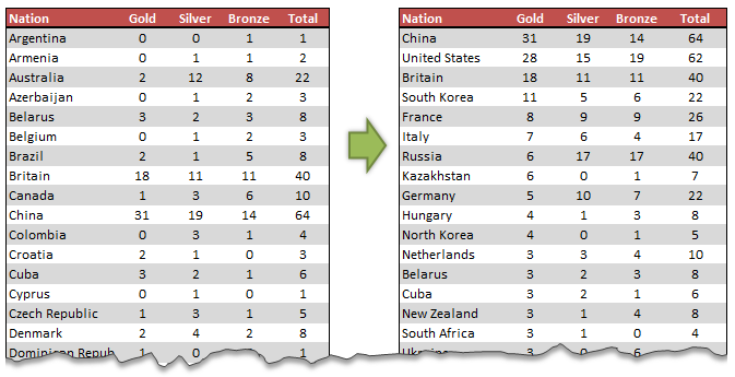
So how do we sort our data in Olympic medal table style?
It is simpler than it looks. All you have to do is use custom sort feature in Excel.
- Select your data
- Go to Home > Sort & Filter > Custom Sort
- Now specify the sort levels and sort orders.
- Click ok and you are done!

Using SORTBY() formula to sort the table
Excel 365 introduced a new formula to sort data by multiple-levels using formulas. SORTBY
Assuming your medal data is in the table named medals you can sort with below formula.
=SORTBY(medals, medals[Gold],-1, medals[Silver], -1, medals[Bronze],-1,
medals[Team / NOC],1)
The -1 parameter tells SORTBY to sort in descending order.
Learn more about SORTBY function & other new formulas in Excel 365.
What if your version of Excel does not have SORTBY
Well, there is a work around. Add an extra column in your data and calculate sort order using a formula, as shown below.
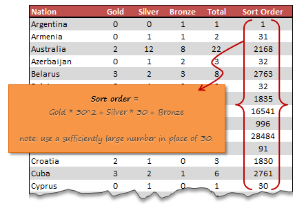
Once you calculate sort order, sort on this column in descending order and you are done.
Video – Sorting Excel data in Olympic medal table style
Watch this short & fun video to learn the sorting technique outlined in this page.
Example file – Olympics Medal Table style sorting in Excel
Please download this Excel file if you want to practice the custom sort or SORTBY() approach.
Do you use custom sort?
Custom sorting is very useful when you 2-3 levels in your data. For example, sorting all projects by department & % completed or sorting all products by region & sales volume. I use it often to understand how my data is.
What about you? Do you use custom sort? What is your experience like? Please share your tips & thoughts using comments.
More Quick Tips on Sorting & Filtering
If you find yourself constantly sorting and filtering, then check out below tips. I am sure you will learn something new.
- Sorting:
- Custom sorting in Pivot tables
- Which formula to use to check if a list is sorted?
- Formula 1 style sorting in Excel
- How to round and then sort data in Excel
- Sorting text values using formulas!
- Shuffling a list in random order in Excel
- How to sort across columns (ie change sort orientation)
- Filtering:
- Filtering values using advanced filters
- How to filter odd or even rows only?
- Right click to filter fast…


8 Responses to “Top 5 keyboard shortcuts for Excel Charts”
As far as I remember (checked, again, 2 minutes ago) in my "Excel 2013" in order to select various chart elements I need to use the Arrow keys and not the TAB key.
Practically, the TAB key does nothing (within a Chart).
----------------------------
Michael (Micky) Avidan
Thanks for pointing this out. This is how I remember it too, but when I was recording the video yesterday, only TAB key worked. MS must have changed the keys in Excel 2016. I have edited the post to include both keys.
The key navigation on charts is different in 2016.
TAB cycles through a layer of objects (SHIFT+TAB cycles backwards)
ENTER move down a layer
ESC moves up a layer
So on a column chart with title/legend/data labels if you select the plotarea the TAB will go through Title > Legend > Plotarea.
ENTER at plotarea will then select Vertical axis. Tab will take you through
Horizontal axis > gridlines > Series > Horizontal Axis.
ENTER with series selected will then allow you to TAB through individual data points and data labels.
If you ENTER on datalabels you can TAB through each data label.
ALT + F1 : to create default chart
ALT+E S T = CTRL + ALT + V, T : I find that easier to remember
I second what Michael already said about TAB and arrow keys. I can't help but think if this is related to the "," or ";" as separator. I prefer to use the chart tools - layout- drop down box, anyway.
Got to be F11 for instant charting. Highlight your data , hit F11 and voila! ?
Ctrl+1 is the most important chart shortcut. In fact, it works for any Excel object: whatever is selected, Ctrl+1 opens the task pane or dialog to format that object.
Somewhere along the line, maybe when Excel 2016 came out, the arrow keys stopped working to cycle through the elements of a chart. But what works is holding Ctrl while clicking the arrow keys. I haven't gotten used to the Tab and other keys, but as long as Ctrl+Arrow works, I'm good.
And F4 used to be so helpful when formatting a lot of charts. But since Excel 2007 came out, it has been mostly useless. It used to remember a whole set of changes at once, so I get that the newer modeless dialogs make that impractical. But now it only seems to work with formatting of lines and borders, and maybe fills. I find myself writing a lot of VBA one-liners in the Immediate Window to handle these tedious formatting tasks.
after clicking on a chart, is there a shortcut key to copy it?
Thank you for the Alt E S T - tip. This is more than a time saver. Because of dynamic charts or de-activated external references to data when you make the charts, you often have empty charts that are otherwise impossible to format. So this shortcut helps adressing that. I will work with it more and see if there remain some obstacles.