

We have some home work folks! Today, lets test your Excel formula skills by giving some data related to a fund.
The problem:
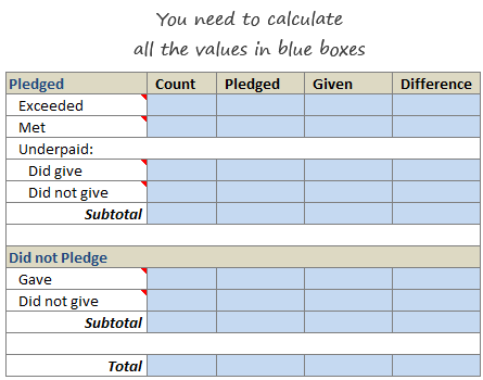
You manage a fund for a non-profit. You have donors who pledge certain amount at the start of the year. As you go thru the year, the donors donate money to your fund. At the end of the year, you have a table like this:

And you need to summarize the fund’s performance by calculating all these statistics.
Download the homework file:
Click here to download the homework file. Write formulas in all blue boxes so that the values are calculated properly.
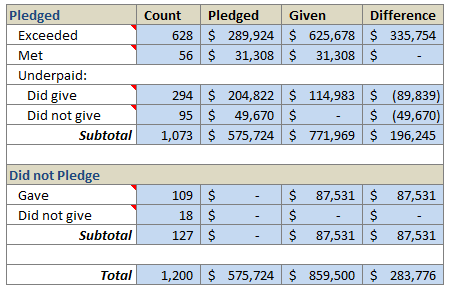
The correct answers are shown below:
Post your Answers using Comments
Once you finish calculating the summary values, please share your approach (and formulas) using comments. Go!
Download the solution file:
There are several ways you can calculate the summary values. Here is my approach. Click here to download the solution file [Excel 2003 version here].
More homework:
If you like to test your Excel skills then, checkout some of these homework problems:
- Calculate sum of digits in a number using Array formulas
- Find average of closest 2 numbers
- When does Thanksgiving day occur on same day again?
- Show zebra lines when value changes
- … More homework & Excel challenges
Thanks David
Special thanks to David, who emailed me this problem a few weeks ago.


26 Responses
Great practice!
First off, I made named ranges – Pledged (C7:C1206) and Given (D7:D1206).
Then it was all about matching the constraints to 0 or 1 and multiplyng them as needed to get the proper sums.
G7: {=SUM(IF(Pledged>0,1,0) * IF(Given>Pledged,1,0))}
H7: {=SUM(IF(Pledged>0,1,0) * IF(Given>Pledged,1,0) *Pledged)}
I7: {=SUM(IF(Pledged>0,1,0) * IF(Given>Pledged,1,0) *Given)}
most of the rest of the array formulas are simply changing the constraints (such as pledged=0 instead of pledged>0), but these other 2 are interesting as well since they need an extra term:
G10: {=SUM(IF(Pledged>0,1,0) * IF(Given0,1,0))}
H10: {=SUM(IF(Pledged>0,1,0) * IF(Given0,1,0) *Pledged)}
I10 doesn’t need the extra term because (IF(Given>0,1,0)) and Given are redundant.
Nice challenge to start the morning! I’m so glad I found this site a few weeks back because it’s great!
I also named my ranges just as Bill did. However, I used a different approach than he and the solution did.
Speaking of the solution – is it correct? Where you got 389, I got 294. Also, when you have 389, the two subtotals equal 1295, so that tells me something is wrong. Here’s what I did:
G7: =SUMPRODUCT((Pledged0))
H7: =SUMPRODUCT((Pledged0)*(Pledged))
I7: =SUMPRODUCT((Pledged0)*(Given))
G8: =SUMPRODUCT((Pledged=Given)*(Pledged>0))
G10: =SUMPRODUCT((Pledged>Given)*(Pledged>0)*(Given>0)*1) // solution didn’t have (given > 0) constraint
G11: =SUMPRODUCT((Pledged>Given)*(Pledged>0)*(Given=0)*1)
G15: =SUMPRODUCT((Pledged=0)*(Given>0)*1)
G16: =SUMPRODUCT((Pledged=0)*(Given=0)*1)
So for the previous 5 rows, the equations in H and I were just multiplied by Pledged and Given, respectively, just like H7 and I7 were.
I also used SUBTOTAL(9,…) for rows 12 and 17 and then SUBTOTAL(9,x7:x17) in row 19.
Is my accusation correct?
Ha! When I posted my solution, it interpreted some things as erroneous HTML tags. My attempt to correct that is replacing > with GT:
.
G7: =SUMPRODUCT((Pledged<Given)*(Pledged GT 0))
H7: =SUMPRODUCT((Pledged<Given)*(Pledged GT 0)*(Pledged))
I7: =SUMPRODUCT((Pledged<Given)*(Pledged GT 0)*(Given))
I’m using SUMPRODUCT for this one:
2 named range:
Amount_Given =Sheet1!$D$7:$D$1206
Amount_Pledged =Sheet1!$C$7:$C$1206
For the first row, exceeded:
COUNT
=SUMPRODUCT(–(Amount_Pledged>0),–(Amount_Given>Amount_Pledged))
PLEDGED =SUMPRODUCT(–(Amount_Pledged>0),–(Amount_Given>Amount_Pledged),Amount_Pledged)
GIVEN =SUMPRODUCT(–(Amount_Pledged>0),–(Amount_Given>Amount_Pledged),Amount_Given)
Where did the 18 names come from for those that did not pledge and did not give?
By my estimate [ Did not Pledge, Did not Give ] should be somewhere around 6.92 billion people.
Good problem, I would have started with the sum(if()) approach and added columns for flags but didn’t have the time to spare for more than a quick review after I saw the No Pledge No donation row.
I have not started yet. but…
pledged = 1168, did not pledge = 127 but total count is 1200? they don’t add up?
First, I added a column next to given called Difference. I then named ranges as pledged, given and dif.
Then I used COUNTIFS() and SUMIFS() formulas to summarize the data:
Row 7: =COUNTIFS(pledged,”>0″,dif,”>0″) =SUMIFS(pledged,pledged,”>0″,dif,”>0″) =SUMIFS(given,pledged,”>0″,dif,”>0″) =J7-I7
Row 8: =COUNTIFS(pledged,”>0″,dif,0) =SUMIFS(pledged,pledged,”>0″,dif,0) =SUMIFS(given,pledged,”>0″,dif,0) =J8-I8
Row 10: =COUNTIFS(pledged,”>0″,given,”>0″,dif,”0″,given,”>0″,dif,”0″,given,”>0″,dif,”0″,given,0) =SUMIFS(pledged,pledged,”>0″,given,0) =SUMIFS(given,pledged,”>0″,given,0) =J11-I11
Row 12: (could have used sum instead, but I continued my formulas down to check my work.) =COUNTIF(pledged,”>0″) =SUMIFS(pledged,pledged,”>0″) =SUMIFS(given,pledged,”>0″) =J12-I12
Row 15 =COUNTIFS(pledged,0,dif,”>0″) =SUMIFS(pledged,pledged,0) =SUMIFS(given,pledged,0) =J15-I15
Row 16 =COUNTIFS(pledged,0,dif,0) =SUMIFS(pledged,pledged,0) 0 =J16-I16
Row 17 =SUM(H15:H16) =SUM(I15:I16) =SUM(J15:J16) =SUM(K15:K16)
Row 19 =SUM(H12,H17) =SUM(I12,I17) =SUM(J12,J17) =SUM(K12,K17)
Good eye Fred – you are right! Chandoo has a mistake in one of the count cell formulas.
Those that did pledge and gave less than the pledge= 294 not 389. Subtotal for all those that pledged and underpaid is 1,073, which makes the total count = 1,200.
Count column results:
Pledged Count
Exceeded 628
Met 56
Underpaid:
Did give 294
Did not give 95
Subtotal 1,073
Did not Pledge
Gave 109
Did not give 18
Row 17 127
Row 19 1,200
using single cell sumproduct formulas for correct conditions
Sorry, should have included this in my previous post. Chandoo’s formula in his cell G10 can be corrected as:
=SUM((lstPledged>lstGiven)*(lstPledged>0)*(lstGiven>0))
(He left off the last condition in the solution spreadsheet.)
Thanks, Chandoo! This was fun work 🙂
okay,
for the explanations, since i cant upload the file
formula in
G7 =SUMPRODUCT(–($C$7:$C$1206>0),–($D$7:$D$1206>$C$7:$C$1206))
H7 =SUMPRODUCT(–($C$7:$C$1206>0),–($D$7:$D$1206>$C$7:$C$1206),C7:C1206)
I7 = =SUMPRODUCT(–($C$7:$C$1206>0),–($D$7:$D$1206>$C$7:$C$1206),D7:D1206)
H10 =SUMPRODUCT(–($C$7:$C$1206>0),–($D$7:$D$12060),C$7:C$1206)
other cells can be manipulated by proper conditions such as pledged > given, = given or < given etc
can be made a bit more elegant by naming the ranges and making it trimmer
My H10 is
={SUMPRODUCT(IF(PLEDGED>0,1,0),IF(GAVE0,1,0))}
and I got 294
Were the 95 people in “Did not give” double counted? Total = 1295 as Fred said
First, “underpaid—did give” count is a miscalculation. it’s simply double counted the 95 just below it (underpaid—did not give). Of course sub totals are not adding up to 1,200.
I’ve done this with array formulas. Here is the link if any one interested.
http://cid-00557615ec1937ba.photos.live.com/self.aspx/Excel%20Public/ArrayFormula.JPG
Remember to press Ctrl+Shift+Enter. Happy Excel every one…!
formula didn’t post right…
H10 should be
{ sumproduct ( if ( pledged > 0 , 1, 0 ), if (gave 0, 1 ,0 ) ) }
and you get 294, then the toal would be correct at 1200
god darn it didn’t post right…
{ sumproduct ( if ( pledged GT 0, 1, 0), if (Gave LT pledged, 1, 0) times if (gave GT zero, one, zero ) ) }
@Fred… Thanks for pointing out the mistake. I fixed it and updated the solution files too. 🙂
Thanks for the donut! 😉
Great task for a Saturday morning – enjoyed doing this a lot.
I started doing this with array formulae, but it got too tricky to debug, so I moved to using sumproduct for the sum columns. In the count columns I used an array formula with the right conditions.
I named the ranges as did most other people, Given and Pledged, then the formulae for the pledged totals (for example) become:
Pledged and Exceeded pledge: =SUMPRODUCT(Pledged, –((Pledged-Given)0))
Pledged and met pledge: =SUMPRODUCT(Pledged, –((Pledged-Given)=0), –(Pledged>0))
Pledged, underpaid but did give: =SUMPRODUCT(Pledged, –((Pledged-Given)>0), –(Pledged>0), –(Given>0))
I’d upload the file somewhere, but I don’t have a website.
Thanks for posting the challenge!
Interesting analysis.
Please find my finished file:
http://cid-18c2ae6c7e70126a.office.live.com/self.aspx/.Documents/formula-homework-donations-calculations.xls
below is everything under the heading count
G7=SUM(($D$7:$D$1206>$C$7:$C$1206)*($C$7:$C$1206>0))
G8=SUM(($D$7:$D$1206=$C$7:$C$1206)*($C$7:$C$1206>0))
G10=SUM(($C$7:$C$1206>$D$7:$D$1206)*($D$7:$D$1206>0))
G11=COUNTIFS($D$7:$D$1206,0,$C$7:$C$1206,”>0″)
G12=SUM(G10:G11,G7:G8)
G15=SUM(($C$7:$C$1206=0)*(D$7:$D$1206>0))
G16=SUM(($C$7:$C$1206=0)*($D$7:$D$1206=0))
G17=SUM(G15:G16)
G19=SUM(G7:G8,G10:G11,G15:G16)
Everything under pledged
H7=SUM(IF($D$7:$D$1206>$C$7:$C$1206,1,0)*C7:C1206)
H8=SUM(($D$7:$D$1206=$C$7:$C$1206)*($C$7:$C$1206>0)*(C7:C1206))
H10=SUM(($C$7:$C$1206>$D$7:$D$1206)*($D$7:$D$1206>0)*$C$7:$C$1206)
H11=SUMIFS($C$7:$C$1206,$D$7:$D$1206,0,$C$7:$C$1206,”>0″)
H12=SUM(H10:H11,H7:H8)
H15=SUM(($C$7:$C$1206=0)*($D$7:E$1206>0)*C7:C1206)
H16=SUM(($C$7:$C$1206=0)*($D$7:$D$1206=0)*C7:C1206)
H17=SUM(H15:H16)
H19=SUM(H7:H8,H10:H11,H15:H16)
everything under Given
I7=SUM(($D$7:$D$1206>$C$7:$C$1206)*(D7:D1206)*(C7:C1206>0))
I8=SUM(($D$7:$D$1206=$C$7:$C$1206)*($C$7:$C$1206>0)*(D7:D1206))
I10=SUM(($C$7:$C$1206>$D$7:$D$1206)*($D$7:$D$1206>0)*$D$7:$D$1206)
I11=SUMIFS($D$7:$D$1206,$D$7:$D$1206,0,$C$7:$C$1206,”>0″)
I12=SUM(I10:I11,I7:I8)
I15=SUM(($C$7:$C$1206=0)*($D$7:D$1206>0)*($D$7:$D$1206))
I16=SUM(($C$7:$C$1206=0)*($D$7:$D$1206=0)*D7:D1206)
I17=SUM(I15:I16)
I19=SUM(I7:I8,I10:I11,I15:I16)
This is for pledged but did not give. The same structure is used in each cell. This makes it easy to read.
=SUM(–
(GIFT[Amount Given]0)*
(GIFT[Amount Given]=0)*
(GIFT[Amount Pledged]))
=SUM(–
(GIFT[Amount Given]0)*
(GIFT[Amount Given]=0)*
(GIFT[Amount Pledged]))
didn’t post properly…
one more try:
“{=SUM(–
(GIFT[Amount Given]0)*
(GIFT[Amount Given]=0)*
(GIFT[Amount Pledged]))}”
{=SUM(–(GIFT[Amount Given]0)*(GIFT[Amount Given]=0)*(GIFT[Amount Pledged]))}