

With Excel 2007, Microsoft has introduced a powerful and useful feature called as Tables. One of the advantages of Tables is that you can write legible formulas by using structural references. That means, you can write easy to understand formulas like this,
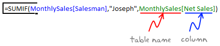
But, there is a problem. When you write these formula and drag the formula cell sideways to fill remaining cells, Excel changes table column references and thus makes your formulas almost useless.
Well, there is a simple workaround for this problem.
Use copy & paste.
Instead of dragging the cell to fill formulas, you can use copy & paste to fill the formulas. In this case, Excel will preserve all table references while changing the cell references accordingly. See this demo to understand:

Share your Table Tips & Tricks
Ever since I discovered the tables feature in Excel 2007, I have been using them to save time and simplify my work with data. Tables have several useful features that make life simple for analysts and data junkies everywhere.
What about you? Do you use Excel Tables? What are your top table tricks? Please share using comments.
More on Excel Tables
If you are using Excel 2007 or above, I encourage you to learn Excel Tables. They will make your life simpler. Go thru below articles to learn more,


11 Responses
If you’re interested to work with Tables from the VBA side of the fence, check out my article on that:
http://www.jkp-ads.com/articles/excel2007tablesvba.asp
I think Tables are the best new feature in Excel 2007, it makes formula building a lot easier once you get the hang of it.
Another workaround for the problem you describe is selecting all three cells in this case and then hit CTRL+R.
I use data tables to create distinct data lists. Copy and paste a column and the Crtl+t to make the pasted column into a table. Then choose to remove duplicates and convert back to a range.
If anyone knows how to use a data table as a validation list it would be very handy
To use a column form a data table in Data Validation list, I use INDIRECT function.
Example: =INDIRECT(“Table1[Column1]”).
Its very handy
@ Tim: to do that you need to create a named range which refers to the column you need from the table.
In the example above if you would want a validation list with the salesmen you would need to create a named range which refers to MonthlySales[Saleman].
Another option would be to use a formula as source for your list in the validation with INDIRECT like =INDIRECT(“MonthlySales[Saleman]”)
@ all
the wonderful 😉 tables also exist in Excel 2003 !
under # Data # List
Regards Stef@n
@ Fowmy; cool, I didn’t know that. It’s strange though that Excel won’t let you use a column from a table as a validation list directly though…
@ Stef@n; the lists in 2003 don’t have all the options as the 2007/2010 tables though. You can’t use the structural references for example.
@ m-b
Refer this link for more info:
http://www.cpearson.com/excel/indirect.htm
some one help me to avoid repetation of lists, when we use =INDIRECT(“Table1[Column1]“) in validation. i.e. I need unique list to be displayed in the validation list.
Thanks
Jude
Tip I learned from ExcelIsfun, Mike Girvin, absolute table reference looks like this Table1[[Field1]:[Field1]]. This one you can drag across without any problem.
Downside, it sure makes your formulas longer.