

Here is a cool count-down timer application made in VBA to remind you about our VBAClasses registration closing time!
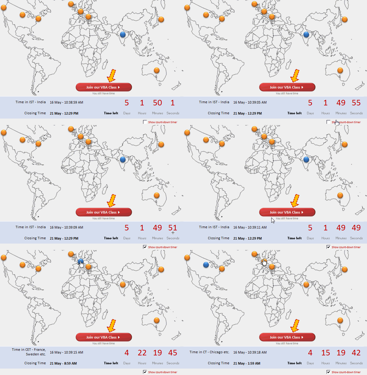
I know it is blindingly awesome. So I will give you a few seconds before reading further.
….
Back already? Great.
I was thinking of ways to tell you that you have got less than 3 days to join our VBA Class. Then it struck me, why not make an Excel workbook to tell you how much time you have got? So I did just that.
Here is a video demo of how the VBA application works (watch on YouTube):
Download the VBA Classes Count-down Timer Workbook:
Click here to download the workbook. Please enable macros to see it.
PS: You must drag and drop this file in to Excel 2007 or above to see it.
How does the Count-down Timer Work?
First, I must tell you about its limitations:
- This workbook assumes that your computer is located at the hotspot (or city) you have chosen.
- The current time is fetched from your computer’s local time using NOW() formula.
Now, the basic construction of this workbook can be broken down to 3 parts:
- Hotspot / City Selection
- Countdown Timer
- Formatting
Hotspot / City Selection:
- I took an outline map of world and put it in an empty sheet. On top of this I have added 9 hotspots by drawing nine circles.
- I have named these hotspots spot1, spot2…,spot9
- As you can guess, each of these spots correspond to one time zone, from PST to Australian Time.
- I have assigned macros to each of them. The macros would just modify a cell named valSpot with the name of the spot on which I clicked.
- Based on the clicked spot, I fetched the corresponding closing time from a table like this:

- Then, I calculated the time left by subtracting current time from closing time.
- A similar logic is used for City selection.
Countdown timer:
- I have inserted a check box and linked it to a cell named showTimer
- I have also assigned a macro startTimer to the checkbox.
- The startTimer macro would call a different macro named – countDownTime()
- In this, I wrote a while loop that would check if the showTimer is true and ask Excel to update the currentTime once every second
- The code can be examined from the downloaded file.
Formatting:
I am leaving this to your imagination.
Bottom line: Join our VBA Classes
Of course, the whole point of this is very simple.
If you want to learn VBA, then please join our VBA classes. We will be closing registrations in 3 more days. After that we will be busy for next few months teaching VBA to those of you who joined us.
Click here to join our VBA Classes.
PS: When you join our VBA Class, you get to learn how this timer app is constructed in a detailed 40 minute lesson. That is just one of the many lessons in our class. So, join us already.


15 Responses
What, no Wellington! Hell, not only did you miss my city out, but my country too 😉
How ’bout replacing all those separate macros with just one:
Sub who_called()hotSpotClick Application.Caller
End Sub
@Jeff… awesome tip on the application.caller. Now, that makes the app even more sexy.
I missed Wellington because it has one hell of a VBA / Excel ninja who is spreading the awareness already.
Hi Chandoo,
Looks awesome. However, when I tried to download it although the hyperlink shows as a “.xlsm” file my system seems to recognize it as a zip file and defaults to downloading it as that.
That means there’s no way of then opening it as far as I can see.
Changing the download suffix to xlsm works fine.
Just thought I’d mention it in case anyone else is having the same problem.
John
Hi, awesome. But i have a problem 🙁 … I can’t open the file. Please help us about it.
Thanks!!
Chandoo,
Please explain what you’ve done here. When I select Los Angeles on the map, it says I have 2 days left but when I select India or Australia, it says I have 3 days left.
I don’t think your spreadsheet is following the GMT correctly. If anything, all the countries in the negative time zone should have more time than the countries in the positive time zone.
Just my feedback but I’d love to know your thoughts.
Awesome tool! 😉
Just one note:
D21 = now() but D20 can change depending on the hotsopt you click. it creates an illusion that all hotspots have the same local time.
Question: how much time does it take to create something like this from draft to finish?
Hi Chandoo,
This is awesome. Very good app indeed.
Small suggestion: Counter is not ticking right from when the app is opened (even though “Show count-down timer is opened).
How about adding this event?
Private Sub Workbook_Open()
Run “countDownTime”
End Sub
Regards,
Ravi.
Dear All,
It is my first post on chandoo.org, my favourite source of Excel solutions. Great work!
@Dennis:
Try to download and save this file “as is” on your desktop or anywhere else and although it is being shown as .zip file, just drag it to opened blank Excel sheet, confirm that you want to open it and… enjoy.
Another way to overcome this problem has been solved by John Pomfret above.
Thank you.
Awesome concept for data visualization. Workbook looks elegant, except for the fact that the times are incorrectly shown.
Keep up the good work!
Not sure how you open this file. I get a zip file with a bunch of xml files. I would appreciate some advice. Thanks.
@All: Thanks everyone for the encouraging comments and feedback.
@Sagar: please note that, the workbook assumes you are located in the hotspot / city you have chosen. So it just calculates the time gap from NOW() and the closing time.
@Fred… It took me a couple of hours to conceptualize this and may be another hour to create it. But the fine-tuning took lot more time and I wasted some time with other variations of same visualization.
@Ravi: Good suggestion on initiating the counter on workbook open. Thanks for sharing it with us 🙂
@For those of you having troubles opening this file: Just save the file on your desktop (or some folder) and then drag and drop it inside Excel 2007 or 2010.
Hi All,
I want to prepare a macro which give me a callback reminder so what would be the correct coding for the same.
e.g if i call on a mobile number today @ 10 AM and he gives me callback time @ 1 PM so i want a pop up come out automatically when clock time reach @ 1 PM
Please help me in this
Regards
Kuldeep Rathore
lstCities
=#REFERENS!#REFERENS!
What is the correct Information ?