
This article is part of our VLOOKUP Week. Read more.
Situation
Often we need our lookup formulas to go wild. Not in the sense of go-wild-and-chomp-a-few-kilo-bytes-of-data sense. But wild like wild cards.
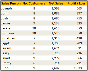
For eg. In the below data, we may not remember the full name of sales person, but we know that her name starts with jac. Now how do you get the sales amount for that person?
Data:
Solution
Simple. Use wild cards. Like this: =VLOOKUP("jac*",$B$5:$E$17,3,FALSE) to fetch the value from 3rd column for the person whose name starts with jac
Examples:

Sample File
Download Example File – Using Wild cards with VLOOKUP formula
Special Thanks to
Michael Pennington, Lukas for the tip. (Click on the name to see their tip)
Similar Tips
- Excel SUMIF and COUNTIF Formulas – What are they, how to use & examples
- Search Workbooks using Conditional Formatting & Wildcards


21 Responses
Hi Chandoo,
To answer the first question we can use VLOOKUP(“*ve*”,$B$5:$E$17,2,FALSE)
This is a great tip, and one I can see applying to other formulas as well. My only concern: what if your wildcard has more than one answer? Vlookup can only handle one response, correct? And it will only return one value (i’m guessing the first record that it encounters where it meets that condition). This could really mess you up if you just assumed it was right – so be careful with Vlookup and wildcards!
Hi Tom
Use this formula as a test if there are more than one values that comply with the lookup (G7 is the first cell of the dataRange and G25 is the last cell o the dataRange)
=ISNUMBER(MATCH(input,OFFSET($G$7,MATCH(input,dataRange,0),0):$G$25,0))
The inner match function finds the position of the first result, the offset function adjusts the starting cell in the range to the cell below that and the second match function finds the position (if it exists) of the second positive result. If positive, it will be a number and the isnumber function will confirm that. You can then wrap this formula in a if formula eg. If( [above test] , “WARNING: More than one result, “”)
Works well with a concatenate too……
=VLOOKUP(CONCATENATE(B10&”*”),A1:B6,2,FALSE)
@dan I
CONCATENATE function is a waste of characters (and since we all hate having to work harder than we have to), especially since you took the shorter (and faster) method of concatenating the words yourself. A shorter, but exact same re-written function would be:
=VLOOKUP(B10&”*”,A1:B6,2,)
If you use the formula =VLOOKUP(“ja*”,B5:E17,3,FALSE) there are 5 possible answers, but the formula returns 2133, which is the first one encountered. Hence using a wildcard with the VLOOKUP formula isn’t something I’ve used in the past, mainly because with a large data set you can’t be sure of the result.
How to make “Jo*” as vlookup value as a range.
=VLOOKUP(“Jo*”,A1:M14,2,FALSE)
The above one will vlookup only for the “Sales Person” contains letter “Jo*”. If i want to vlookup value for “Je*”, “Ae” & “Co*”. How i can do.
Cannot figure out the Question 3 of the Homework problem, can someone please help.
thanks
PM
PM,
I copied and pasted the number of customers (column ‘D’) to the right of the Name column, and then did a normal vlookup formula.
Best,
Alan
not able to figure out the solution for 3 rd of downloaded file , can u pls healp me
Please help me on 2nd QUestion in Downloaded file.
2. Who made more sales – person ending with ph or starting with je?
Here are my solutions. Feedback appreciated!
1. 2277
=VLOOKUP(“*”&G17&”*”,B5:E17,3,FALSE)
2. Joseph
=INDEX(B5:B17,MATCH(MAX(VLOOKUP(“*ph”,B5:E17,3,FALSE),VLOOKUP(“je*”,B5:E17,3,FALSE)),D5:D17,0))
3. 726
=VLOOKUP(INDEX(B5:B17,MATCH(6,C5:C17,0)),B5:E17,3,FALSE)
Hello,
Just reading through this thread and I was wondering if anyone was able to help with a similar query. I am trying to use a wildcard on a string of numbers but when using the vlookups above it keeps returning N/A.
Below are my tables, I want to look up F1 in A1:A5 and return anthing that contains the 3 numbers.
This is what I have been trying to use:
=VLOOKUP(“*”&F1&”*”,A1:A5,1,FALSE)
Table 1
A1 Acc number Acc name
A2 2356161 Bob
A3 2165151 Sam
A4 4313621561 James
A5 46146143 Sarah
Table 2
Search code
F1 161
F2 143
Any help is much appreciated.
Thanks
1. 1. How many sales for the person whose name contains the text in G17
Ans: 2277
Formula: =IFERROR(VLOOKUP(CONCATENATE(“*”&$G$17&”*”),$B$5:$E$17,3,FALSE),”Error”)
2. 2. Who made more sales – person ending with ph or starting with je?
Ans: Joseph –
Formula: =IFERROR(IF(VLOOKUP(“*ph”,$B$5:$E$17,3,FALSE)>VLOOKUP(“je*”,$B$5:$E$17,3,FALSE), VLOOKUP(“*ph”,$B$5:$E$17,1,FALSE), VLOOKUP(“je*”,$B$5:$E$17,1,FALSE)),”Error”)
3. 3. What is the netsales for the person who had 6 customers?
Ans: 726
Formula: =IFERROR(VLOOKUP(INDEX($B$5:$B$17,MATCH(6,$C$5:$C$17,0)),$B$5:$E$17,3,FALSE),”Error”)
Now, I’m confident about #1 and #2 above. I don’t think #3 is correct. There are actually two people (Jessy and Jimmy) with 6 customers. However the forumla only finds Net Sales for Jimmy only (since VLOOKUP only returns value for the first match it finds). The real answer should be 1440 (adtrer adding 714 for Jimmy). Can someone share the correct formula?
Thanks in advance,
Dear Nil,
Sum ifs can be used “=SUMIFS(D5:D17,C5:C17,6)”
I need to use an if statement with vlookup and a wildcard, is this possible? it is looking at a cell to reference a table to get the terminal location.
=IF($A$26=”@ ATM Deposit 0492*”,VLOOKUP(“@ ATM Deposit 0492*”,$A$2:$B$18,2,FALSE),IF($A$26=”@ ATM Deposit 0494*”,VLOOKUP(“@ ATM Deposit 0494*”,$A$2:$B$18,2,FALSE)))
Very good post. I am using this trick with countif and sumif.
Hi
I replied to a comment aboe befoe realizing the comment was from 2010, lol
Just for those concerned about the problem that there may be more than one result for the wildcard lookup (or also regular lookup) I think you can use this formula as a test if there are more than one values that comply with the lookup (in the example G7 is the first cell of the dataRange and G25 is the last cell of the dataRange – you could also replace these with index funtions eg. Index(dataRange,1,0) for the first and Index(dataRange,COUNTA(dataRange)+COUNTBLANK(dataRange),0) for the last )
Here is the test:
=ISNUMBER(MATCH(input,OFFSET($G$7,MATCH(input,dataRange,0),0):$G$25,0))
The inner match function finds the position of the first result, the offset function adjusts the starting cell in the range to the cell below that and the second match function finds the position (if it exists) of the second positive result. If positive, it will be a number and the isnumber function will confirm that. You can then wrap this formula in a if formula eg. If( [above test] , “WARNING: More than one result, “”)
My cell (A2) contains text separated by company details within cell like IBM;Wipro;Infosys; and I need a formula to display result as Yes if cell has companies other than IBM. If the cell has only IBM; IBM; IBM, result should show up as “No”. Can you help please? I spent 4+ hours without luck 🙁