
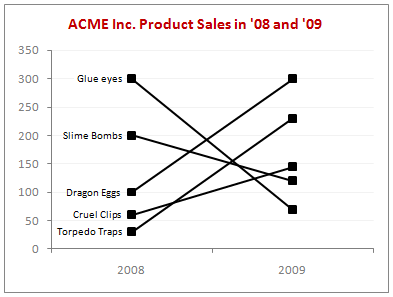
Yesterday I read about interaction plots on junk charts where he points out the merits of an interaction plot. Interaction plots show interaction effects between 2 factors. For eg. you can show how your product sales have changed between year 1 and year 2 using an interaction plot like below:
As you can see, interaction plot is a simple line chart with several series. You can easily make this in Excel. Here is a simplified tutorial to help you get started.
Step 1: Select the data and insert a line chart
This is simple, just insert a line chart from the data.
Step 2: Go to the line chart “data” and change rows to columns
You require this step only if your data is oriented differently.

Step 3: Format the interaction chart
Since excel colors each line series differently, you need to change the colors, add labels, adjust the label source (from data to series) and then format grid lines etc.
That is all, your interaction plot is ready to go.
Download interaction plot template for excel and play with it
Click here to download the interaction chart template for excel and use it to make your own interaction plots.
Points to consider when you are making interaction plots,
- Interaction plots can be too messy if you have a lot of series. Generally they loose the appeal after 6-7 series of data.
- Chart formatting with more series of data can be a pain too. Use F4 key if you are found repeating same steps.
- Make sure you don’t color individual series differently. You can use same color and label instead. It looks a lot better that way.
- In cases like last year vs. this year or budget vs. actual, you can even use clustered bars. See more examples on budget vs. actual charts for inspiration.
What is your opinion about interaction plots?
I think they are good for small data samples. I have personally not used them, but I like the idea and will use them when there is an an opportunity. What about you? Have you used them in any professional setting? How did your audience feel about the chart? Tell us using the comments.


8 Responses
If you have many series, you could split the chart into multiple panels, as in the example in How to Build a Simple Panel Chart.
Hi Guys,
Should this chart be a table…
Nice post. You’ll find interaction charts are used a lot in the biomedical sciences to show when changes in particular outcomes, let’s say the effect of a drug, are dependent on other factors, for example age or sex.
Jon, I absolutely agree that panels make for a really time efficient and data rich method for visualising interactions across many variables.
Ross, I’m not sure about a table beingt he best option. To me, the chart would help the reader understand the nature of the interaction much better than a table. A table with a sparklines/microcharts may be even better. I suppose it comes down to what question you’re answering with the chart. Are you more interested in the exact figures (in which case I totally agree with you) or is the main story the interaction (in which case I’d go with the charts or table with sparklines).
@Jon.. good suggestion.
@Ross: yeah, you can make a table, As AoverT pointed out, tables lack visual appeal, so chart might more effective to prove a point.
@AoverT: Very good remarks. Thanks for sharing your experience.
Chandoo,
you wouldnt’ know how to do that version of interaction chart easily in excel
http://flowingdata.com/2009/11/10/do-we-need-more-teachers/sat-scores/
Do I miss sth or is it really necessary to fake the axis through dummy series? i’m not seeing the forrest for the trees right now
@Chris… I think you have to fake the axis thru dummy series. Good link btw.
Oh, it is cool information. Will try it. thanks
Hello, thank you for your explanation!
I was wondering if it was possible to have on the same graph (and the same columns) another point indicating the mean and also SEM?
Thanks!!