
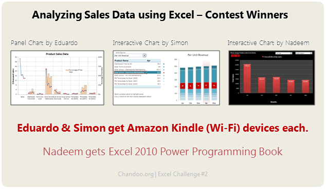
Winners of Sales Analysis Chart Contest:
Yesterday we saw the entries for the sales analysis chart contest. Today, we will find who the winner is…,
Oh, wait!
I have decided to award the prize to 2 contestants. Each of them will get an Amazon Kindle Reading Device.
The winners are,
And there is a third prize too. This will be Excel 2010 Power Programming Book by John Walkenbach.
The winner is,
- Nadeem (Option 31)
Congratulations to the winners.
Also, all the participants of this contest will receive a small surprise bonus. Wait for it until this weekend.
PowerPivot T-shirt Giveaway
Recently, I got an email from Emilie, a member of PowerPivot (review) team at Microsoft, who promised to do backflips if I promote their PowerPivot Contest. I did promote the contest (here). But she went back on her backflips promise and instead sent me a 4 PowerPivot t-shirts. They are really cool. But, unfortunately, I cannot wear all of them.
So I am going to give away these 3 shirts (shown below).

How does this giveaway work?
- I can only send these shirts to addresses in India.
- To participate, just post a comment on this article. Anything goes.
- The shirts are in Girls L, Girls M, Guys L sizes.
- This contest closes on 3rd July, 11:30 PM IST (Indian Standard Time, we are GMT +5:30)
- What are you waiting for? Go!
That is all for now. I will see you next week with more Excel awesomeness. You have a beautiful weekend then.


40 Responses
aaaah, pity that I’m from slovakia
Sad didnt got Kindle…..Looking forward to get at least this T-Shirt and Surprise prizes…
Congratulations to the 3 winners and Congratulations to All who participated.
Hui…
hey, you said no macros!! #41 has macros!
This is gonna be PowerPivot Awesome T-Shirt 🙂
Hip Hip Hurray !!!
Regards
Rohit1409
M happy I am atleast in Top 3 & m getting Power Progamming Book.
Thanks Chandoo.
@Shellie – I think he had written not to use macro’s to create chart & we misunderstood that we cannot use macro’s in the sheet. I had also used 1 macro only to change formatting of chart after selecting dropdown.
Lets see who gets Powerpivot Tshirt :p
Hey,
Liked the solutions…lots of new ideas …………but somehow liked Nadeem’s solution than others
Chandoo,
Perhaps you would consider sharing the rationale behind why the three winning charts were chosen in the order they were so readers gain additional insight.
@Chandoo: #41 used Macro’s..Your take on this??
” “
Chandoo, T shirt belongs to me because this is my first comment in your website 🙂
Hmmm interesting Tee… send me the Men’s L 🙂 … I am from bangalore 🙂
This PowerPivot t-shirt might turn out to be only reason after which my wife don’t cry over me glued to maze of jails where numberes are captured – my wife’s interpretation of spreadsheet 😉
Contest was really great… I learnt lot of new approach of looking at the data set. Keep more coming in…
Great contest! The downloads are a course all on their own. By the way, I really need a tee shirt. I just lost 30 lbs. (hee hee).
Congrats to the winners. You guys really inspire us..
Shirts looks great! too bad they wont fit me (need XL)…if I win
Hi Chandoo, L size fits me so well. Also my gf says that color black turns her on, so please help 😉
Hello Chandoo,
I really liked your post about PowerPivot. It gives users the power to create compelling self-service, facility of sharing. It is owesome. It works great. I hope everyone will should know about this. And Chandoo your PowerPivot T-Shirts are very cool & attractive. Would that I get this T-Shirt.
Thnx for posting about the PowerPivot.
Thnx & Regards,
Karan
Congrats to all winners and all those who participated.
Really cool entries.
Chandoo, btw, if possible blue tshirt please : )
Thanks,
Herman/ Delhi
Want my Powerpivot Awesome T-Shirt !!
Yipee…. Chandoo – L size does it for me 🙂
You Guys Rocks …. Thanks for teaching this king of stuffs
Congrats to winner……..but I belive nadeem’s chart were most impressive…….
Congrats to all winners bt smthing is nt fair
#41 has used macro – how can he win.
I think #31 should have win this.
I also want tee shirt. For tht wt shd i do ?
Thanks Chandoo for the great website and excellent stuff on excel. You have really made learning excel a fun and thrilling experience.
I work in the field of analytics and would love to get the PowerPivot tshirt (Men L).
Hello Chandanna,
I came to know about you from First edition of ET Wealth dated Dec 13 2010. The Article Titled ” Work Excel ” is a big source of inspiration for me and i thank you for unraveling the secrets of Excel with mind blowing concepts , ideas , homework & Contests. It’s like All creative brains under a single roof.
Thank you for being a source of inspiration for digging Excel.
Suresh
Visakhapatnam
Hi Chandoo
simply i need de tshirt (men L)
thanks plzzzzzz give to me
guru
i will accept the fact that i am going crazy… looking at these charts… you will not believe, that how much i gained (and at times effortlessly….by using the charts you all posted)…. Using creativity and inputs from you all, i would like to post that i am earning goodwill at office. and i am proud to say, i DO COPY from this site…. But let me assure you, that i do use my creativity too…. thanks all for such wonderful posts… And NO WORDS to thank Chandoo for his site and selections…………. what can i say… JUST HATS OFF !!
Just a question on Nadeem’s chart. When I change the drop down on the left to percentage both drop downs disappear for me. Does that happen to others on here?
Congratulations to the winners.
I like L size black T-shirt. 😉
hey chandoo!
I wanna have the Tee! Send me one!
@Zilla
When this dropdown is changes I have attached a small macro on it to change the data labes from $$ to %age. So might be your macros are disabled.
Or else, I have prepared this chart in Exel 2007 & in case you are using Excel 2003 – Charts behave little different in xl 2003 when prepared in xl 2007.
This chart is working smoothly on my home & office pc.
Please confirm if some1 else is experiencing same problem – I will try to lookout for Bugs.
Contest still open??
If so i would like the Girls m sizr (for my gf).
Also better chance of getting 😛
Just downloaded a project remplate from this site. Been my first visit … but a fruitful one ! I’m going to come back often for more useful stuff. Way to go Chandoo !!!
Dear Chandooooooooo,
I am not here for T-shirt but i gain lot of knowledge because of your site as well Charting i am using exclusively.
Must mention that you are doing very fabulous job. Keep it up !!
Rajnikant
Oops … Am I late here ?
Chandoo, it’s not fair ! 🙂 You wished us to have a beautiful weekend and I literally had one, on a trip with my college friends in western ghats of Karnataka !
And here I am , an avid follower of your blog.
Hope I get a chance to get that tee 🙂
Cheers !
Damn…..The only Excel Comptetion of Chandoo where i had a shot….And so many comments…
Congratulations to the Winners
I saw and learned from this website. I found many intresting chart that can amazingly made from excel especially from nadeem. But I think of something that should be more concidered. that’s about the use of each chart, e.g : we use pie chart for percentage; we use cluster bar chart for overall comparison (product monthly). but beside of that, thax for inspiration
Dear sir,
Appreciate and let me have the file