
 While preparing a project plan, I had a strange problem. I wanted to highlight all the project tasks that fall with-in a certain date range. At the lowest level, the problem is like this:
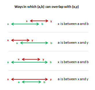
There are 2 ranges of dates (a,b) and (x,y) and I want to know if they overlap (ie at least one date common between a,b and x,y)
The formula for testing such a thing seemed tricky at first. So I drew the conditions on paper to get clarity on what we should test. Evidently, there are 4 ways in dates (a,b) can overlap with dates (x,y) as shown below:
Now, we can test for the overlap condition using a formula like this:
If x is between a and b

or a is between x and y

then overlap

else do not overlap
As you know, there is no formula in excel like isbetween(). So we have to break it up to 2 conditions and an AND() Formula. Finally the formula becomes,
=if(or(and(x>=a,x<=b),and(a>=x,a<=y)),"Overlap","Do not overlap")
Now, it seemed like quite a big formula for testing if 2 ranges of dates overlap.
So, I continued my quest for even shorter formula.
After sometime, I realized that if we test for non-overlap instead of overlap, we can write a shorter formula.
Do not understand? Let me explain.
While there are 4 ways in which (a,b) can overlap with (x,y), there are only two ways in which (a,b) cannot overlap with (x,y). See this to understand:

Now, testing above conditions is very straight forward in excel.
the formula becomes, =if(or(y<a,b<x),"Do not overlap","Overlap")
The formula is much shorter and easy to maintain.
I was able to use it to test if a set of tasks in the project plan are running between given dates (for eg. next week). All is well in the end.
How do you test overlap conditions?
Do you ever have to test overlap conditions? What kind of formulas have you used? Please share your formula tips & tricks using comments.


62 Responses
a good example to illustrate how clear thinking leads to simple solutions!
this illustrates very well how clear thinking leads to simple solutions!
Chandoo,
Yes, I’ve done this before. My solution is very similar to yours.
To use conditional formatting to highlight a cell when ab and xy overlap, just enter this formula in the Conditional Formatting Rules Manager:
=NOT((y<a)+(b<x))
Regards,
Daniel Ferry
excelhero.com
I built a form where you can input both ranges and it generates a conditional format using match formula. Blue where a value matches another one in the other range and Orange if it could not find a match.
I don’t have much to add for once, suffice, as they would say in Boston, you are wicked smart
You can test for the overlap (rather than the non-overlap) more easily than you did:
=if(and(x<=b,a<=y),"Overlap","Do not overlap")
A little longer than yours, since I used <= and you used <, and AND has one more character than OR. But it may be easier to understand without the NOT.
If you just want to highlight the cells—- then why not use two Conditional Formatting commands (Excel 2007) for the range of cells you want to test.
Highlight Cells between XXX and XXX.
x is between a and b
a is between x and y
This is my first post and I just want to say thanks to you and your community that make regular posts—you and they—-inspire me to take my game to the next level.
I have a couple of workbooks that I check for overlaps. I will be changing them and applying your solution as its easier to understand and a bit brilliant. Followed your link to Excel Hero’s article “I heart IF” (thanks) which was really enlightening. Based on that, you could use : REPT(“Overlap”,(a<=y)*(x<=b))
There is also a function published in mrexcel:
http://www.mrexcel.com/forum/showthread.php?t=346005&highlight=character+number
Public Function IsBetween(testvalue As Variant, lwr As Variant, upr As Variant, Optional equaltype As Boolean) As Boolean
If equaltype Then
IsBetween = (testvalue >= lwr And testvalue lwr And testvalue < upr)
End If
End Function
Amazing! I wrote a similar post two days ago. I have to admit your formula is much better!
Just curious. In your data, are always a<b and x<y?
I can remember early in high school learning about Sets, Intersection, Outersections and Logicals (and, or, not etc) and thinking “why would I ever need to use these ?”
To analyse these types of problems, that why.
Another way could be =if(min(y,b)<max(x,a),"Do Not Overlap","Overlap")
Little longer than your formula, but I like this for the flexibility it can offer when you want to check this for 3 dates ranges 🙂
I use the same basic formula as Vipul. I compute OL = min(y,b) – max(x,a), where OL is the amount (i.e., length) of the overlap. If OL > 0, the intervals overlap and OL gives how much they overlap. If OL <= 0, they do not overlap (and OL gives how far apart the closest ends of the intervals are).
Thank you soo much for this Nick for the min/max idea. This post really helped me solve my problem. In my case (a,b) remains stationary (e.g. 1/1/2017, 1/1/2018). However, the length of (x,y) varies between days and years in all 4 of the scenarios.
I needed to calculate the length of overlap time to help me calculate proportion of the average (in my case number waste packages produced between x and y) that falls on the overlap.
I used {min(y,b)-max(x,a)/(y-x)}*total no. of packages (produced between x and y). y-x gives the total length of time and min(y,b)-max(x,a) gives the fraction of overlap.
Thank you Chandoo for the x,y and a,b modelling, it really helped me solve my issue.
🙂
@Daniel.. very good way to shrink it even further.
@Gregor, Alex, Alan, Oscar, Rick — Thank you … you are welcome 🙂
@Jon .. Interesting.. now why didnt I think of that…
@Pavel.. yes. In almost all plans (except one involving time machines), start date is less than end date.
@Hui… most of what we do in our work traces back to elementary stuff we learn in school.
@Vipul and Nick.. Thank you so much for sharing your tips..
@Adison: I would be very keen to use your form. If possible, mail it to me – chandoo.d @ gmail.com
Interesting ideas. I use a slight variation of Jon’s formula:
=if(and(x=a),”Overlap”,”Do not overlap”)
The advantage of the slight change is as follows. The above formula (as do the others above) reports an overlap if the time periods are adjacent (e.g. one ends @ 4PM and the other starts @ 4PM on the same day).
Sinece the 4PM end/start points are an “instant in time”, there is technically no overlap. If you want to exclude adjacent segments of time from the overlap test, simply remove the = sign from the two expressons above:
=if(and(xa),”Overlap”,”Do not overlap”)
Of course, this second formula will not report an overlap even if the four values are identical!
Sorry, my previous post was corrupted. The two formulas should be akin to the following:
IF (X IS LESS THAN OR EQUAL TO B) AND (Y IS GREATER THAN OR EQUAL TO A)
OVERLAP
and
IF (X IS LESS THAN B) AND (Y IS GREATER THAN A)
OVERLAP excluding adjacent times.
This is great and works in most cases for me – being a complete novice with Excel I have encountered a problem with the formula =if(or(y<a,b<x),"Do not overlap","Overlap") I can't solve.
If I have two lists, xy and ab (where x and a define the lower limit of a range and y and b the upper) and I apply the formula such that I'm checking whether the value in the range defined by ab is present in the list of ranges defined by xy the formula doesn't work in the case that list ab is longer then list xy. In this case I get a #VALUE! returned in the formula cell for every case where the values in ab are below the list xy – why is this?
What about sorting the data first ,,, sort the data by Machine number then use an IF statement =IF(C4=C3,IF(E4>D5,”Not OK”,”OK”),””). This easy use of an IF statement returns OK if the dates do not overlap and Not OK if the dates do overlap and also checks to see if the machine numbers are the same and if they are not the same number then it leaves the space blank as it is the start of the next machines task.
Thanks, Chandoo, for that clear and concise explanation at the beginning. I had been struggling with this problem for days until I came upon this page. I have a long list of overlapping ranges (associated with genetic info) and wanted to find out how many other ranges in the list overlap each test range row. I used the following approach:
=218 – (COUNTIFS(F$2:F$219,”less than”&E2) + COUNTIFS(E$2:E$219,”greater than”&F2))
where there are 219 rows, F$2:F$219 contains all the start coords of the ranges (the x’s and a’s in your example) and E$2:E$219 contains all the end coords (the y’s and b’s). The countifs sum is subtracted from the total number of rows minus one to avoid counting the row being operated on (at least I think that’s why).
Anyway, thanks again for your original post.
-Rob
By the way, I also meant to add that I could use help from the panel on the next challenge which is to return the row numbers of the overlapping rows. At this moment, I don’t know exactly how to approach this. I’m thinking that vlookup might work somehow, or maybe an array function. Any ideas?
Vaguely wandered across this post while double-checking my logic for exactly this issue. Since I was looking at creating a UDF to be used in the VBE, rather than a worksheet formula, I thought I’d throw this in the mix too:
Public Function dateRangeOverlaps(firstStartDate As Date, firstEndDate As Date, _
secondStartDate As Date, secondEndDate As Date) As Boolean
dateRangeOverlaps = Not ((secondEndDate < firstStartDate) + (firstEndDate < _
secondStartDate))
End Function
I liked Post #20 and used it, only to realise it tells you, for each range, the total number of overlaps.
I am looking for the total number of ranges that span a given day.
I suppose I could adapt #20 by making a long column with days from min to max, but that seems ugly. How can I generate a range of days in a formula?
Excellent description, was really useful.
What was the formula solution to this? I cannot find a soution anywhere! Would really appreciate it.
I have a related problem, but I think that it is a step more involved. I do not know if I can solve it with a single formula or array formula, or I should do it “long hand.”
I have a number of monthly periods in adjacent columns – headed by dates e.g. 31/1/2013, 28/2/2013, 31/3/2013 etc.
I have separately a table of “deals” which specify Start date, finish date, and capacity utilisation. e.g. 2/1/2013, 3/3/2013, 10MW; 14/1/2013, 10/2/2013, 20MW…
What I want to do is to check, for each monthly period, what is the maximum capacity utilisation in that month?
So I need to check, for each month, the sum of capacity utilisation on individual deals where there is any overlap between the deals.
I realise that I could do this by doing a sheet with 365 columns, or I could run some macro, but I thought it might just be possible to calculate this within one formula. Any thoughts?
Where can I wire the beer?
For clarification, I wanted to specify my question a bit better: … What I want to do is to check, for each monthly period, what is the highest total capacity utilisation at any time in that month?
I am reading your posts and it really is helping me in my research!
I have a small question:
What if we want to count the number of days that is overlapped if overlapped?
Which formula would be best to use in this case?
My question falls along these lines.
I have two date ranges A through B, and X through Y.
I need to conditionally format a cell if any dates in range A-B fall within range X-Y.
Thanks for this!! I needed a simple solution and you came through. I was able to use this in a non-Excel format, thanks to your clear explanations.
I have formula to identify overlap dates but i want to pull which data is overlap please tell me how to do this
I use this formula to identify overlap or not
=SUMPRODUCT((G3=$B$3:$B$100)*(F3=$A$3:$A$100))
Thank you so much for this!
Was searching exactly for this type of formula to calculate overtime overlap in a time-sheet.
Perfect!
Hi
Can any one tell me what is SQL query for Overlapping dates in range to pull all the data
hi chandu
i need your help i am having process wise start date&time & each process hours. my shit time is 9to 6 hours. some times the workers are doing before 9 o clock overtime some time after 6 they will done overtime. so i need that cummulative overtime in hours.
I am just learning how to write formulas with functions like IF and AND in Excel. I often find your articles very helpful – thank you.
Two questions: 1) Am I misunderstanding something? Shouldn’t your third variety of overlap be “y is between a and b” not “x is between a and b”, which is your first option?
2) Can you apply this formula to more than two rows, and get the values of the overlap, not just a true/false type of result?
I am, like Rob, dealing with ranges of genetic markers, in my case, for genealogy. Each row shows a match between two people, which is an overlapping range of numbers. There are 3 columns of data for each match: chromosome number, start position, end position. I sort it by chromosome number and start number. The numbers start over for each chromosome, so the formula has to start over too.
Using your idea of visualizing the problem as a physical overlap, I managed to create formulas using IF and AND to identify pairs of rows with overlapping data ranges, and even to return the start and end values of that overlapping range. However, I can’t figure out how to get the start and end values for overlaps involving more than two rows. I think it might take an array formula.
This data is only useful for genealogy if you can “triangulate” it – that is, at least three people overlap in the same range, and you already how two of them are related. The bigger the overlap, the closer they are likely to be related. The more people who overlap in the same range, the better – if you know the relationship of one or more match in a set, it helps you identify the others. So it’s important not just to identify whether or not there is an overlap, but exactly what the numbers are.
An example:
Match 1 – A vs B: Start 1, End 30, nephew
Match 2 – A vs C: Start 3, End 15, rel. unknown
Match 3 – B vs C: Start 12, End 18, rel. unknown
Match 4 – A vs D: Start 19, End 29, known cousin
(No Match – B vs D, C vs D)
I can eyeball this and see that the only range that the first three overlap is 12 to 15. But how do I write a formula to do this? And a conundrum: Match 3 overlaps 1 and 2, Match 4 also overlaps 1 and 2, but 3 and 4 do not overlap each other.
Other issues: These numbers range from 1 to millions. There are other parameters that weight the data. Over time I will be adding people to my database as they do DNA tests and share results with me. This is a dynamic process.
Should I even try to do this with formulas?
I’m trying to write a formula that will only alert the user if there are more than 4 overlaps and less than 3. Simply put, I want there to be 3-4 workers scheduled at any given time. Any idea what the simplest formula would be to achieve this?
Thank you in advance!
Checking one date range to a handful of others is fairly straightforward.
However, is it also possible to check all the date ranges in a list for overlap with each other? Say for example you want to identify which days in the calendar are accounted for in a list of date ranges and identify which dates have overlaps and/or are duplicated in the various range entries.
BN
Yes it is possible:
http://www.get-digital-help.com/2015/05/20/count-overlapping-days-in-multiple-date-ranges-part-2/
I am attempting to adapt this to fit my need but I am missing something here. In my sheet I have a chart that is designed to tell me a list of events (A10-A24) and the quantity of equipment needed, ie Laptops (C10:C24) for a given range of times – equipment drop times (G10:G24) and equipment collection times (H10:H24). So for example: Registration (A10) requires 1 laptop (C10) from 7:00 AM (G10 formatted as a time) to 8:30 AM (H10 is also formatted as a time).
The goal of this chart is not just to tell me quantities of equipment needed and when, it also needs to tell me how many of each piece of equipment I should have on hand for that given day. My logic is that if I can calculate – per row – how many times other events overlap the time range of that row, I can SUM the equipment requested (Column C) for the given row and ever row that has a timing conflict. Then just take a max of that output, which would tell me for example how many laptops I’ll need to have in the field at a given time.
I was using:
=SUMIFS(C10:C24, G10:G24, “>=”&G10,G10:G24,”<="&H10)+ SUMIFS(C10:C24, G10:G24, "=” &G10)
Which I know is incorrect because it is just adding the output of the two SUMIFS. I feel like I am close to figuring this out but something is missing. Any Advice? Thanks for your time.
I am Looking for similar formular where I am having Multiple employee and sengle employee having multiple Start date and end date, wanted to check whether each employee having a overlapping date range.
Not able to formulate
Not able to figure out how to built a formula
Your formula ONLY works if the 1st time starts before the 2nd time. I’m in need of a formula that checks it both ways. Like your first picture. I have to do 2 timesheets and sometimes one start time is before the other, sometimes it’s after. In other words 7am-8am & 8am-9-am (ok, that’s after). But then other times it’s the other way around. I’m speaking sheet one and sheet two. Let’s take the other way around one and say I have a brain lapse. So I’ve put 8am-9am on sheet one and 7:30am-8:30 on the other. This formula won’t catch it. I have to put in a second column >’s in the formula for it to catch it. But then I have two columns. One that says overlap and one that says do not overlap. So I still have to check it. It also says overlap in the cells that are empty.
Hi all,
Not sure if you could help me, but it’s worth a try. I need to calculate something which seems a bit more complex than just identifying if there is an overlap.
In my project management dataset I have a project which has a standard number of days to finish the project (in this case 13 weeks * 7 days = 91 days (SLA)). Sometimes, there are delays possible which block the delivery of the project. These delays are registrated based on a start- and an enddate. the number of days could be identified via enddate – startdate. I add this number of days to the original SLA date. Unfortunatelly, it is possible to have multiple delays which could influence the delivery, even in the same time, but I do not want to double the effect of lost days.
To make thinks more complex, I could have 3 delays reported in a project which I should take into account in this formula. Next to that, I have to take into account that not all delay categories should be taken into account for this delay checker.
Does anyone have a solution for this problem, or might give some guidence?
Thanks!
@JB
I’d suggest posting the question in the Chandoo.org Forums
https://chandoo.org/forum/
Attach a sample file with an example if you can so you will getr a more targeted response
You saved my day! You have explained as simple as possible. Great!!
Hi Chandoo,
I appreciate your straight Mat thought and I have been having problem with some overlapping events: I would like to calculate each even’ts non-overlap minutes from a time series of downtime events.
A generic formula supposed to work for any duration of a time event condition such as multiple events overlap, some, non etc. Up to that point no problem but when total duration of some random events overlap with a single event then I am having issues in terms of a generic excel formulation to calculate non-overlap time of each event. That sheet will be automated so I can’t use different formula for each row since when sheet gets updated all new downtime will be on it. Here is an example:
If you specifically look up 12/14/2017 8:00 am to 12/15/2017 9:00, you can see my point.
Downtime Start (with date) Downtime End (with date)
12/14/2017 6:00 12/14/2017 7:30
12/14/2017 6:30 12/14/2017 7:30
12/14/2017 6:30 12/14/2017 16:00
12/14/2017 7:00 12/14/2017 8:15
12/14/2017 7:30 12/14/2017 8:30
12/14/2017 7:30 12/14/2017 15:00
12/14/2017 7:45 12/14/2017 8:00
12/14/2017 8:00 12/15/2017 9:00
12/14/2017 9:00 12/14/2017 10:00
12/14/2017 11:00 12/15/2017 16:00
Your help would be really appreciated!
Thanks
G.S
Brilliant post, love the logical approach, so easy to pick up and re-use. And to think, I was reading other posts and looking at nasty QUERY functions for such a simple task… Thanks
This was so helpful, thank you for this simple breakdown!
Hey there Excel pro’s,
Loved the post and comments!
Any idea how to apply this concept to a range?
I.e.
I have 20 items with start and finish dates. There are three item types.
I want to ensure that each start and finish date does not overlap with another start and finish date of the same type item.
The table columns looks like;
Item type ; Item ; Date start ; Date end
Thanks for making the web great!!
Cheers,
Bill
Your initial formula
=if(or(and(x>=a,x=x,a=a,x=x,a<=y)),(AND(xb))),”yes”,”no”)
For example: If you build a project plan in Excel, so you have column D (start date), E (end date) and then K10-AH10 has the first day of the week listed (ex. 1/6, 1/13, 1/20…). Now on each row in K-AH you want the cells to color block like a ghant chart to show if the start/end dates fall within the chart dates in K10-AH10. If you use this formula:
=IF(OR(AND($D38>=L$10,$D38<M$10),(AND($E38L$10)),(AND($D38M$10))),”yes”,”no”)
Then drag it down with autofill for the “ghant” area. Then select the entire area and apply conditional formatting so that if “yes” then black text & black fill color, if “no” then white text & fill color. – Now you have made your own ghant chart with the date ranges you need to represent in Excel that auto-update for you as the project changes.
Chandoo, thanks for that.
I have a challenging one for you or someone that can find a way to solve it.
I have 20 rows of different activities, each row/activity has a start location and an end e.g. Excavation from 2.3 km to 3.3km. Each km is in a different cell.
Can you think of a way (formula) to conditional format it so I can quickly identify if there are any activities that are taking place within the same area (clashes)?
Hopefully you can solve it, mate.
Thanks.
Thanks a lot.
It is very useful.
Very nice. Thank you!
for the first formula, this:
=if(or(and(x>=a,x=x,a<y)),"Overlap","Do not overlap")
would be more accurate.
the reason being that if x=b, or if a=y, then it is not an overlap, but is succession.
something went wrong when copy pasting, so heres the correction:
=if(or(and(x>=a,x=x,a<y)),"Overlap","Do not overlap")
Thank you. Great thinking. Great explanation. Great solution. Much appreciation.