• Hi All

    Please note that at the Chandoo.org Forums there is Zero Tolerance to Spam

    Post Spam and you Will Be Deleted as a User

    Hui...

  • When starting a new post, to receive a quicker and more targeted answer, Please include a sample file in the initial post.

Table populated with subset of another Table, without using Pivot Tables

k1s

Member
Hi I've got a feeling I'm missing something very simple, but would appreciate help

I'd like to create a table that is a subset of an existing table, but I don't think a pivot table or Advanced Filter are going to work

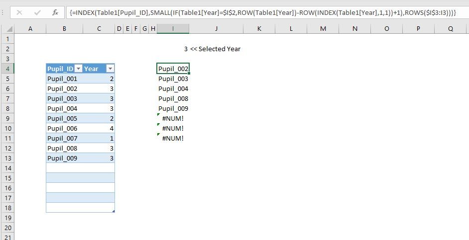
In Table_1 I have a column 'Pupil ID' and a column 'Year'.

In Table_2[Pupil ID] I want the column to contain the Pupil IDs from Table_1[Pupil_ID] where there is a "3" in Table_1[Year]

Clipboard01.jpg


Table_2 needs to be automatically populated, and I need to it to be able contain other data from Table_1, correpdonding to the Pupil ID.

An Index & Match array formula doesn't seem to work because Table_2 is a proper table which doesn't allow array formulae.

I tried creating a data relationship but that didn't work because some of the cells in Table_1[Pupil ID] are blank and an error message indicates thinks these are duplicate values.

Any tips greatly appreciated
 
{=INDEX(Table1[Pupil_ID],SMALL(IF(Table1[Year]=$I$2,ROW(Table1[Year])-ROW(INDEX(Table1[Year],1,1))+1),ROWS($I$3:I3)))}

^^ Array Formula

chandoo_zpspastuash.jpg
 
Hi Paul, thanks for your reply, but as far as I understand it, a Table won't accept an array formula.
 
This is very similar, but includes looking up additional columns. I defined the array as a formula and got away from needing an array function.
 

Attachments

  • SortEx.xlsx
    12.3 KB · Views: 32
FYI - Table does accept array formula.
upload_2016-12-19_18-40-22.png
See attached.
 

Attachments

  • SampleTableArray.xlsx
    13.3 KB · Views: 23
Thanks Mike, I was indeed going to go on and pull the other columns,

I've converted it to use structured references, but the trouble is, using this approach, a new entry in Table_1 doesn't automatically appear in Table_2. - see attached
 

Attachments

  • SortEx2.xlsx
    14.4 KB · Views: 7
FYI - Table does accept array formula
I guess I should have said it won't accept multi-cell array formulae... (which is probably why I couldn't get it to automatically update Table_2 once a new pupil is added is added to Table_1)
 
Last edited:
Thanks Mike,

...why not just use the column filters in the first table?
The first Table is the database and has >382 fields/columns. I'm trying to use Table 2 will be a data-entry table for some of those fields. Tables 3-n will be dashboard reports with some slicers, to make viewing/analysing the data more manageble.

I was thinking there was probably a way to do this using the data modelling "Connections"/"Relationships" features in Excel but I have no experience with these.

Anyway a combination of that code you found and Chihiro's array, means I don't need to use the named range, but I can't get the Table_2 to resize because my VBA is not very good.

How can it be adjusted to ignore the #N/A rows in Table_1[Pupils]?

Also is there a way to use structured references so that I don't have to specify the worksheet location of the tables or absolute cell references in Table_2?

Code:
' THINGS TO CHANGE IN THE CODE:
' "Sheet1" - name of Worksheet that holds "Table_1"
' "Table1" - if not named "Table1", change all "Table_1" in code to correct name
' "Sheet2" - name of Worksheet that holds "Table_2"
' "Table2" - if not named "Table2", change all "Table_2" in code to correct name
' Range for "Table_2" - in the place below where you have $A$1:$D, change the $D to
'                      the last column in "Table_2"
Option Explicit
Private Sub Worksheet_Change(ByVal Target As Range)
    Dim delRows As Long
'
Application.EnableEvents = False
' See if Table1 and Table2 now have different row counts
    delRows = ActiveWorkbook.Worksheets("Sheet1").ListObjects("Table_1").ListRows.Count - _
                    ActiveWorkbook.Worksheets("Sheet1").ListObjects("Table_2").ListRows.Count
    If (delRows <> 0) Then Call UpdateTable2(delRows)
Application.EnableEvents = True
'
End Sub
Sub UpdateTable2(AddRows As Long)
    Dim i As Long
    Dim nRows As Long
'
    nRows = ActiveWorkbook.Worksheets("Sheet1").ListObjects("Table_2").ListRows.Count
    If (AddRows > 0) Then
        ActiveWorkbook.Worksheets("Sheet1").ListObjects("Table_2").Resize Range("$g4:$k$" & nRows + 1 + AddRows)
    ElseIf (AddRows < 0) Then
        For i = 1 To -AddRows Step 1
            ActiveWorkbook.Worksheets("Sheet1").ListObjects("Table_2").ListRows(nRows + AddRows).Delete
        Next i
    End If
End Sub
 
Unfortunately, VBA is not my strong point. Hopefully one of the excellent VBA people on this forum can help further.
 
Thanks John,

So we're counting the number of rows in the first Table in a column that doesn't have #N/A, and only adding a row to the second Table if it doesn't take us over that total.

Ingenious.

When I add a row to Table_1, say with Pup011 and Year 3, it adds it in to Table_2, but only if there are already spare rows in Table_2 (which I'm trying to avoid). Is there a way to make Table 2 resize automatically to the right number of rows - i.e. value in G3 in your example?


Hi to all!
Note: If you get Excel 2013 or Higher, you can add a Slicer to tables.
 
Is there a way to make Table 2 resize automatically to the right number of rows - i.e. value in G3 in your example?

There are several ways to do it. Could be with PowerQuery, or a Macro Event. This time, I show you how to do it with a Macro Event.

Check the file. Blessings!
 

Attachments

  • SortEx2.xlsm
    19 KB · Views: 14
Many thanks John. I'm trying to understand some things in the code. In particular, I don't understand what this does:
Code:
If Intersect(Target, .ListObjects("Table_1").Range.Columns(2)) Is Nothing And _
            Target.Address <> "$L$1" Then GoTo Fin

Would you mind explaining / outlining the Power Query route (if it's not too much to ask)? I've just used it for the forst time yesterday and not very confident with it yet.
 
Hi k1s.

Many thanks John. I'm trying to understand some things in the code.

First, sorry for my english. I'll try to explain.

This part means that the code only works if the cell of change is the second column of the Table_1, or if is the cell L1. If is another, the code not updates the resultant Table.

I attach another file with two solutions: First with Macro Event and Second with PowerQuery. Basically is a merge between two queries (each table is converted to a query). When you change something, just right click into resultant table (Table_4) and click Refresh. Blessings!
 

Attachments

  • SortEx2.xlsm
    29.5 KB · Views: 14
Thanks for the explanation John, and thanks for the PowerQuery example.

Using PowerQuery - will it always need refresshing or is there a way to automate it?

(I'm going to have to spend some time trying to get to grips with powerquery so that I can work out how it could be adapted for the actual tables I'm going to use.
 
Thanks for the explanation John, and thanks for the PowerQuery example.

Using PowerQuery - will it always need refresshing or is there a way to automate it?

Yes. With another Macro Event code. Check file. Blessings!
 

Attachments

  • SortEx2.xlsm
    31.1 KB · Views: 8
  • Like
Reactions: k1s
Hi John,

I'm trying to go a step further, so that it can extract records based on multiple "OR" criteria. So in the example attached it would be in English"

List all the Pupils who scored 2 or lower in any of the Tests, and then show me the test and the score

Clipboard01.jpg


I'm not really sure how that would work with the count-based solution you worked up before. Would greatly appreciate some help.
 

Attachments

  • Copy of SortEx5.xlsm
    40.5 KB · Views: 5
I think I've nearly solved it inspired by Chihiro's unpivot suggestion, here, and then filtering the Table in PowerQuery to exclude the values I didn't need ("3 " in this example)

A question though: Is there a way to have it filter, based on the value in a cell on the sheet: H1 in this case? Perhaps in the advanced query somehow?:
Code:
let
    Source = Excel.CurrentWorkbook(){[Name="Table_1"]}[Content],
    #"Changed Type" = Table.TransformColumnTypes(Source,{{"Pupil ID", type text}, {"Test 1", Int64.Type}, {"Test 2", Int64.Type}, {"Test 3", Int64.Type}, {"Something Else", type text}}),
    #"Unpivoted Columns" = Table.UnpivotOtherColumns(#"Changed Type", {"Pupil ID", "Something Else"}, "Attribute", "Value"),
    #"Renamed Columns" = Table.RenameColumns(#"Unpivoted Columns",{{"Attribute", "Test"}, {"Value", "Score"}}),
    #"Reordered Columns" = Table.ReorderColumns(#"Renamed Columns",{"Pupil ID", "Test", "Score", "Something Else"}),
    #"Filtered Rows" = Table.SelectRows(#"Reordered Columns", each ([Score] <> 3))
in
    #"Filtered Rows"

Here's what I did:
Select cell in Table_1
From Ribbon: Data > From Table
In PowerQuery:
Select 3 test Columns
Ribbon: Transform: Unpivot Columns
Filter Score column to exclude "3"
Rename columns
Ribbon: Load & Save to…
(Interestingly when I opted to Load it to the existing sheet, PQ wrongly said the "The selected range is in a different workbook. Please select a range in the existing workbook.", so I had to opt for New Worksheet and then cut & paste to the correct sheet)
 

Attachments

  • SortEx6.xlsm
    120.8 KB · Views: 5
To reference value stored in sheets via PowerQuery, you'd need to put it in either named range or table.

For single value, I'd recommend going named range method.

First name the cell like "fval".

Now go to your PowerQuery advanced editor. Add following line below "let".
Code:
FilterVal = Excel.CurrentWorkbook(){[Name="fval"]}[Content]{0}[Column1],

Then edit your #"Filtered Rows" line to something like below.
Code:
#"Filtered Rows" = Table.SelectRows(#"Reordered Columns", each ([Score] <>FilterVal))

Edit: Remove unnecessary "." after CurrentWorkbook
 
Last edited:
Hi, thanks, the advanced editor is saying: "Expression.SyntaxError: Invalid identifier."

Seems to be underlining "Excel.CurrentWorkbook"

Clipboard03.jpg
 
Back
Top