Replicate data across cells in a staff leave planner [SOLVED]

[paulstan]

Sorry about subject title. Couldn't think what else to call it.

I posted not long ago regarding this Planner and I have now stumbled upon another problem. Spreadsheet attached.

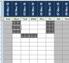
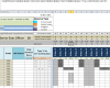
In simplistic terms what I am trying to do is when entering 'x''s in columns H:L (non-working days), I would like the corresponding day of the week to be automatically annotated with an 'x' across the entire year of the Planner (as per the red 'x''s I have manually input). If these had to be entered manually, it would be an extremely
time-consuming job, with potential for errors.
I say 'simplistic terms', but I gather it probably will not be. I've looked at counting cell Colours in conditional formatting ranges, but to no avail.
Any help would be greatly appreciated. My main goal is to have the figures in rows 12 and 13 reduce by the number of 'x''s entered - so, just count the staff who are actually in work.
ps. All macros have been removed.

Thanks for taking the time to look at this.

Regards

Paul S

 

[Luke M]

Formula in P33:
=IF(IFERROR(HLOOKUP(TEXT(P$32,"ddd"),$H$32:$L33,ROWS($H$32:$L33),0),0)="x","x","")

Copy down and across as needed.

Also, formula in P13 can be simplified to:
=COUNTIFS($D$33:$D$42,"SEO",P33:P42,"<>x")
Copy across.

 

[paulstan]

Luke

Thanks for your reply. Unfortunately, the formula copied across the Planner would not allow for manually entring data for instance, Leave (letter 'A'). Is there anything that could be added to the Conditional Formatting which would add the 'x' and still count it as a non-working day?

I have simplified the formula at P13, which works fine.

Regards

Paul

 

[Luke M]

Ok. How about using the hashmark pattern fill?

CF with a formula of:
=IFERROR(HLOOKUP(TEXT(P$32,"ddd"),$H$32:$L33,ROWS($H$32:$L33),0),0)="x"

Appearance:

Can change color if you want.

Formula in P13 then would need to change, perhaps to:
=SUMPRODUCT(($H$32:$L$32=TEXT(P32,"ddd"))*($D$33:$D$42="SEO")*($H$33:$L$42<>"X"))

I don't know what the formula in row 12 is supposed to be calculating, but I'm guessing it'll need to change as well.

 

[paulstan]

Luke

That is fantastic. Looks like it works.

I've simplified Row 12 to
=(R13/100)*R8 - I will do away with the column showing 'left section'.

Finally, this works great if the non-working days are uniform across the year, ie someone doesn't work any Mondays, of which Column H would contain an 'x'. What I would also like to do is have an irregular non-working day (say, someone doesn't work every third Wednesday) and this is signified by the letter N (see Absence Type legend on spreadsheet). I would want to manually type an 'N' onto the Planner for the specific Wednesdays and then have the staff count reduce by 1 at Row 13.

Regards

Paul S

 

[Luke M]

Can change formula then to this:
=SUMPRODUCT(($H$32:$L$32=TEXT(P32,"ddd"))*($D$33:$D$42="SEO")*($H$33:$L$42<>"X"))-COUNTIF(P33:P42,"N")

Or, if you are going to be using lots of different letters for other items, but just want to deduct any marking, could do:
=SUMPRODUCT(($H$32:$L$32=TEXT(P32,"ddd"))*($D$33:$D$42="SEO")*($H$33:$L$42<>"X"))-COUNTA(P33:P42)

 

[paulstan]

Luke

That is fantastic.

Many thanks for all of your help - you certainly know your stuff.

Regards [SOLVED]

Paul S