• Hi All

    Please note that at the Chandoo.org Forums there is Zero Tolerance to Spam

    Post Spam and you Will Be Deleted as a User

    Hui...

  • When starting a new post, to receive a quicker and more targeted answer, Please include a sample file in the initial post.

Making use of array formulas in UDFs

GreggR

New Member
I love the power of array formulas in spreadsheets, however my question is:

Can I utilise this same power in a pure VBA User-defined Function?

I have had a good look but can't seem to find how to do it?

In my current use case, I want to do an INDEX/MATCH multi-value lookup. This screen shot shows a very simplified version of my actual spreadsheet:

excel-array-function.jpg


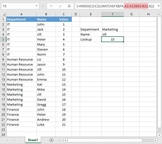
The magic I am trying to emulate happens in the shaded part of the formula in the above image: "A2:A22&B2:B22" which takes the two arrays and returns a single array with each item equal to the concatenation of the corresponding item in the original two arrays.

If I have two arrays of same length in VBA, I can't find how make this same magic happen.

Note that I do NOT want to construct a string formula and place it in a spreadsheet. My goal is to do everything in VBA and just return the found value.

I know I can easily do this with For loops, but the data table can become very large (many tens of thousands of rows) and I want to make use of the lovely optimised code built into the guts of Excel rather than slow VBA loops.

I need this function to work as fast as possible as I will be using it to create other large tables with potentially thousands of uses of the function and that's why I am exploring all the options.

Basically I was hoping this simple looking code would work (but it fails):
Code:
Function LookupDepartmentName(department As String, firstName As String)
    'Trying to convert {=INDEX(C2:C22,MATCH(F3&F4,A2:A22&B2:B22,0))} to VBA...
    LookupDepartmentName = WorksheetFunction.Index(ActiveSheet.Range("C2:C22"), WorksheetFunction.Match(department & firstName, ActiveSheet.Range("A2:A22") & ActiveSheet.Range("B2:B22"), 0))
End Function

I have a VLookup version working but it requires an extra column to be added to pre-calculate the lookup keys and I'm trying to avoid having to do that:
Code:
Function LookupDepartmentName(department As String, firstName As String)
    'NOTE: This assumes a different spreadsheet from that shown above
    '  It would need a pre-calculated column of lookup keys inserted before column A
    LookupDepartmentName = WorksheetFunction.VLookup(department & firstName, ActiveSheet.Range("A2:D22"), 4, False)
End Function

So, is there a way to perform these magic array formulas in pure VBA?
 

Attachments

  • upload_2018-8-22_21-7-33.png
    upload_2018-8-22_21-7-33.png
    42.5 KB · Views: 6
Yes. Use Evaluate rather than WorksheetFunction.

Though it is slightly slower method. It handles array function without issue.

Have a read of link below for detailed article on the topic.
https://fastexcel.wordpress.com/201...to-make-excels-evaluate-method-twice-as-fast/

How do you intend to use it though? If you are going to fill range of cells with the UDF... I'd not recommend it, as it's actually slower than standard formula.

Another approach is to use named range to hold formula and/or dynamic range.
 
Thanks for your speedy reply, chihiro.

I had not come across Evaluate so this is now a part of my Excel arsenal…thanks.

I read it and worry that although you say "slightly slower" it would turn out to be more than slightly slower, with all the string concatenation required to build the formula. Remember, our UDF will be used thousands of times in a single sheet.

We are attempting to create UDFs for our users, who are NOT Excel Power Users.

Here is an ACTUAL example of the array formula I had to create to get the desired result:

=INDEX($H$4:$H$7683,MATCH($E4&$F4&$I4&$D4,$E$4:$E$7683&$F$4:$F$7683&$I$4:$I$7683&$D$4:$D$7683,0))

There is no way our users could cope with that so our goal is to turn that into:

=LookupAvg1($E4,$F4,$I4,$D4)

I know UDFs are slower than standard formulas and that's why I'm trying to determine the fastest version of a UDF, given the vast difference in complexity of the above two examples.

Even if everything was a named range, the INDEX/MATCH option would still be too complex for our client base. And they'd still have to understand/remember to press Ctrl+Shift+Enter.
 
Last edited:
Is the use case confined to the specific workbook? I'd also recommend uploading sample workbook. It's much easier for us to give sample solution with it.
 
Well no. We'd like to make these UDFs available to all open workbooks.

I appreciate your assistance and have uploaded my testing workbook with dummy data.

Am off to bed now but will answer any questions you may have about the workbook tomorrow.

Again, thanks.
 

Attachments

  • lookup-test.xlsm
    590.3 KB · Views: 3
We'd like to make these UDFs available to all open workbooks.

But that defeats the purpose of creating such UDF. Unless all workbooks have exactly the same range that need to be iterated over. You'd still need to define those in the formula as well.

Since lookup range will most likely change from workbook to workbook. I'd recommend setting up Named Range for each workbook.

Add 3 named ranges mylookup1 to 3. And use that as lookup function.

But in my opinion, if you want to make it simple for user. Then introduce helper column to perform lookup operation.

i.e. add column to concatenate conditions.

Or just set up Pivot Table with slicer controls. But best method, will depend on use case for the retrieved value.

See attached for named range version.
 

Attachments

  • lookup-test.xlsm
    605.3 KB · Views: 3
I haven't really got to the task of determining the best way to make it available to all active workbooks.

I think your comment was a result of me not setting up the sample spreadsheet in a clear way.

I used the data table itself for the arguments to the UDF calls. This was just for my own testing purposes and will not be the reality. The arguments will come from other tables (and different table for different sets of calls).

That means your neat named range formulas will not work in this case because the lookup_array arg in the MATCH function is positional but we need to be able to supply args from anywhere.

Regarding the helper function, yes I would say that's the front runner at the moment. I was just hoping to avoid the extra setup required for that method.

So, to get back to my initial question...

Can anyone tell me if it's possible to emulate the wonderful array formula feature available in spreadsheet functions in pure VBA as described above?

If so, what is the syntax?

If not, I think my question is answered but appreciate all the assistance given.
 
Here is code for a UDF using Evaluate:

Code:
Function LookupEval(pp As Long, ss As String, dd As String, mm As String, RtnCol As Long, Optional DRange As Variant) As Variant

If IsMissing(DRange) Then Set DRange = Range("$D$4:$I$7683") ' Or use named range as default
With DRange.Columns
  LookupEval = .Parent.Evaluate("=INDEX(" & .Item(RtnCol).Address & ",MATCH(""" & pp & ss & dd & mm & """," & .Item(1).Address & "&" & .Item(2).Address & "&" & .Item(3).Address & "&" & .Item(6).Address & ",0))")
End With
End Function

Times for returning 3 columns from the first 500 rows, using the data in your uploaded spreadsheet are:
Array formula: 0.74 s
Index/Match: 1.40 s
UDF VLookup: 4.10 s
Named Range: 0.84 s
Eval UDF: 6.4 s

So the UDF is slower, but not so slow as to make it unusable.

I will tidy up the spreadsheet, and upload it with a separate message.
 
Interesting analysis. Not thoroughly tested but i think a couple of points discussed in the recent blog post may be relevant here also:

1. For x2 performance a leading plus sign could be used in place of the equals sign within the Evaluate formula (unary plus just dereferences the result).

2 Activesheet range references can be replaced by references to the calling sheet so that, for example, pressing Ctrl+Alt+F9 with another sheet active doesn't display an error. i.e.:

Application.ThisCell.Worksheet.Range(...)
 
Lori, Doing some timing (with Excel 365 and Windows 10):

Starting the evaluate formula with a "=" or "+" doesn't seem to make any difference.

.Parent.Evaluate seems to work just as well as Worksheets("Sheet1").Evaluate, and avoids the hard-coded sheet name.

But yes, the code as written didn't work if the data range was not supplied, and the sheet was recalculated with another sheet active, so I have added Application.ThisCell.Worksheet., but really hard-coding the range is not a great idea, so I have converted it to a table, so the default data range becomes:
If IsMissing(DRange) Then Set DRange = Application.ThisCell.Worksheet.ListObjects("Table1").Range

Updated file attached.
 

Attachments

  • lookup-test-Eval.xlsm
    520.6 KB · Views: 2
@Doug Jenkins

Yes, 'LookupEval' works whichever sheet is active now. Making the same replacement in the other 'LookupAvg1','LookupAvg2','LookupAvg3' functions also works for them too.

Interesting the behaviour is different in Office 365, on my 2016 set up the udf runs approx 50% faster with the "+INDEX(" substitution.

I find Evaluate("test()") appears to evaluate the udf 'test()' twice but sheet1.Evaluate("+test()") only evaluates it once (tested by writing to immediate window - Charles Williams made this observation with the prefix "0+")
 
I have updated the spreadsheet:
"= Index" changed to "+Index" since this is still faster in some versions
Lookup1 modified with a RtnCol argument, so you can use it to return any column, and an optional Drange argument, with "results2" as the default range.

Just a reminder that the times are for looking up 500 results. Time for 1 is near instantaneous for all options.
 

Attachments

  • lookup-test-Eval.xlsm
    565.7 KB · Views: 4
Back
Top