You are using an out of date browser. It may not display this or other websites correctly.
You should upgrade or use an alternative browser.
You should upgrade or use an alternative browser.
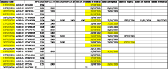
highlight in yellow if within same month
- Thread starter shili12
- Start date
shili12
Member
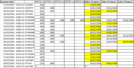
office 365, the other data was retrieved using FILTER, observed your worksheet, on issuance dates its highlighting all cells, instead of leaving them void of colour. Maybe i can filter them out like this, its our person who issued certificate from main portal in feb 2024 but we cant see settlement for the same in statement. however there is possibility of typo errors and account indicated as agents name, too.


Last edited:
p45cal
Well-Known Member
Perhaps he did:Did you look at the solution I offered you at all? Your subsequent posts suggest not.
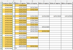
on issuance dates its highlighting all cells
Marc L
Excel Ninja
According to the initial post attachment without any CF a VBA demonstration to paste only to the worksheet module :
Code:
Sub Demo1()
  Const F = "IF(ISNUMBER(Q#:U#),IF(MONTH(Q#:U#)=MONTH(I#),ADDRESS(#,COLUMN(Q#:U#))))"
    Dim L&, R&, V
        L = UsedRange.Rows.Count
        Application.ScreenUpdating = False
        Range("I2:I" & L & ",Q2:U" & L).Interior.ColorIndex = xlNone
    For R = 2 To L
        V = Filter(Evaluate(Replace(F, "#", R)), False, False)
        If UBound(V) > -1 Then Range("I" & R & "," & Join(V, ",")).Interior.ColorIndex = 35
    Next
        Application.ScreenUpdating = True
End Sub
Do you like it ? So thanks to click on bottom right Like !
shili12
Member
yes, i did, i tried it out and even sent you a screenshot of how i would circumvent, as colour was reflected in all cells, none excepting. see #4Did you look at the solution I offered you at all? Your subsequent posts suggest not.
I even carefully saved the file, as its bound to save me hours and hours of work thru visual checking, which may not be possible with larger files.
Marc L
Excel Ninja
which may not be possible with larger files.
With such files avoid CF …


