• Hi All

    Please note that at the Chandoo.org Forums there is Zero Tolerance to Spam

    Post Spam and you Will Be Deleted as a User

    Hui...

  • When starting a new post, to receive a quicker and more targeted answer, Please include a sample file in the initial post.

Get labels based on colors

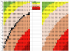
Hello, I have a table of heat stress indicators from column H to column AA. Column AE contains the names of the colors in the indicators table. I want the names in column F, given the numbers in column E, as they are written manually. Thank you.
 

Attachments

  • New Microsoft Excel Worksheet (5).xlsx
    23.4 KB · Views: 4
for yellow for example - you cannot use between 71 and 80 - as the table looks like its not that simple

23.5 Temp and RH of 70 = a THI of 72 - and is coloured YELLOW

BUT
24 Temp and RH of 70 - a THI of 72 - BUT this is coloured PINK

so i guess you cannot setup 6 rules in conditional formatting to say
if column E is between 71 and 80 ie a rule like
AND ( $E2 > = 68 $E2 <= 81 )
then format YELLOW

it will have to do a grid lookup and pick the fill colour - which will need VBA

unless all the THI numbers in a range are all the same
like red again some a 90 but others are orange

i cannot help with VBA

but if the table was to be colour for all the same numbers - then it would be simple
6 rules - 1 for each colour and a formula in conditional formatting could be used
LIKE
AND ( $E2 > = 68 $E2 <= 71 )

BUT you have a few outliner extras ....... so it cant do that
 
so if you replaced all the grid , instead of a THI number you had the name - then it would be easy , as it woul dbe a grid lookup
which can be done in lots of ways - like xlookup / index-match - etc

depending on what version of excel you have

BUT like the colours - the names will be different depending on the same issue
23.5 Temp and RH of 70 = a THI of 72 - and is coloured YELLOW
BUT
24 Temp and RH of 70 - a THI of 72 - BUT this is coloured PINK

otherwise you will need VBA to find the FILL Colour and then lookup the fill colour on the names list

23.5 Temp and RH of 70 = a THI of 72 - and is coloured YELLOW , and MILD STRESS
BUT
24 Temp and RH of 70 - a THI of 72 - BUT this is coloured PINK, and SERVER STRESS

if you had the same table again but instead of THI numbers - you had the words - again easy

others may know a better way to do this - I can only thing of VBA

in fact you could just have a list of numbers and the stress

0​
64​
NO STRESS
68​
MILD STRESS
72​
SEVER STRESS
80​
VERY SEVER STRESS
90​
DEAD COWS
99​
DEAD COWS

And use that with a less than lookup
xlookup or index/match

BUT 72 is across the bounday of 2 colours

would you be able to setup a table like that

even easier -


i'm away for a couple of days now - so hopefully another member can help
 
Last edited:
added an edit for a simple table
if THI numbers can be made up like

0
64NO STRESS
68MILD STRESS
72SEVER STRESS
80VERY SEVER STRESS
90DEAD COWS
99DEAD COWS
 
Assuming you can reconcile so things like 72 does = two different stress levels etc
as i mentioned above


then
a table like

0​
Below Threshold
64​
NO STRESS
68​
MILD STRESS
72​
SEVER STRESS
80​
VERY SEVER STRESS
90​
DEAD COWS
98​
DEAD COWS

would work with
see column G

=XLOOKUP(E2,$AD$2:$AD$8,$AE$2:$AE$8,"Not Found",-1)

should work

as you have Dead cows twice then you may as well remove that

and just have - as anything 90 and above is DEAD COWS

0​
Below Threshold
64​
NO STRESS
68​
MILD STRESS
72​
SEVER STRESS
80​
VERY SEVER STRESS
90​
DEAD COWS
 

Attachments

  • New Microsoft Excel Worksheet -ETAFxlsx.xlsx
    24 KB · Views: 1
On phone in cafe
So
=XLOOKUP(E2,$AD$2:$AD$8,$AE$2:$AE$8,"Not Found",-1)

In older version use

Index($ae$2:$ae$8,match(e2,$ad$2:$ad$8,1))

But you have not said about the different stress words for the same number

As say in a cafe
So away most of today
 
Back
Top