• Hi All

    Please note that at the Chandoo.org Forums there is Zero Tolerance to Spam

    Post Spam and you Will Be Deleted as a User

    Hui...

  • When starting a new post, to receive a quicker and more targeted answer, Please include a sample file in the initial post.

FIFO Cost calculation with Let and Lamda Formula.

Dear Excel Genius,
As per the below snapshot the formula is working and I calculated the cost of RM1 by using the formula
=LET(q,M4:M8,p,Y4:Y8,s,Z4:Z8,sa,SCAN(0,s,LAMBDA(a,v,SUM(a,v)))-s,qa,SUM(q)-sa,
by,BYROW(SCAN(0,q,LAMBDA(a,v,a+v)),LAMBDA(v,LET(qa,v-sa,SUM(IF(qa>0,IF(qa>s,s,qa))*p)))),by-IFERROR(SMALL(by,SEQUENCE(ROWS(q),,0)),))

Above formula provided by the below-linked post Thanks to @Excel Wizard


Attached the file sheet name costing.
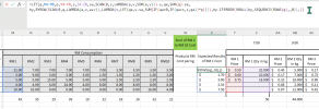
snbGDPJ12q.png

Now, the new sheet named Costing New has 3 companies RM consumption N:N Price AA:AA and the Qty AB:AB.
Company name mentioned in the column B and Z. I transfer the same formula but there is a error of Spill.
After correcting the error I need the costing of each row with the specified company name.
Company A consumption N:W must use company A price and Qty in the column AA and AB respectively.
Likewise, I need Y column results as per the company A, B, C
RM1 purchase price and Qty of A company must use the same company consumption only.

For example I added 5 rows of A then B then C in line. But actually all consumption, Price and Qty will get random Entry too.
likely AAAABBBCCCAACCBBAACBA....etc. So in the formula need to take care of this too.

Here I request you to correct the error in the formula as well as RM1 Cost must be extracted by company wise too.

Thanks in advance.
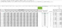
EXCEL_ZvFogvONsN.png
 

Attachments

  • Excel Wizard Solution Chandoo.xlsx
    26.1 KB · Views: 4
There appears to be problems with your use of relative referencing. Absolute references (ideally defined names) would be more meaningful.
I have introduced a Lambda function to your model and, as far as it goes, it appears to check out.
I do not understand whether your records for companies A, B and C imply that there are separate product flows for each company or whether all transactions for one company were complete before dealings with the second company started.
 

Attachments

  • Excel Wizard Solution Chandoo.xlsx
    31.1 KB · Views: 3
@Peter Bartholomew Thanks a lot for your effort towards my post.

The error of spill was sorted out and company A cost of RM1 is correct.

However, the costs of companies B and C are not exactly what I expected.

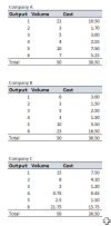
The A total RM1 volume is 47, but the purchase is 50. The remaining 7 must be in stock. Whenever A gets volume, these 7 are used, and until then, they will stay in stock only. They should not be used for B, C, or D.

B RM1 consumption volume 6, 3, 5, 3, and 10 / Price and Purchase 22kg by 0.5$, 10kg by 0.6$, and 18kg by 0.75$

So the cost of Company B RM1 is below

6*0.5=3$
3*0.5=1.5$
5*0.5=2.5$
3*0.5=1.5$
and the last 10kg used 5*0.5=2.5$ + 5*0.6=3$
So the RM1 cost is 2.5+3=5.5$

Likewise C company too.

Volume 15, 8, 2, 0.75, and 2.5 / Price and Purchase 22kg by 0.5$, 10kg by 0.6$, and 18kg by 0.75$

15*0.5=7.5$
7*0.5=3.5$ + 1*0.6=0.6$ = 4.1$
2*0.6=1.2$
0.75*0.6=0.45$
2.5*0.6=1.5$

ABC... represents projects underway in various locations within a single company. I need to compute the costs for RM1 to RM10 individually.

For instance, the consumption volume for Project A should only consider the price and quantity from A. Similarly, Projects B and C should calculate their respective costs based on their own price and quantity data.
 
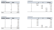
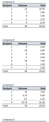
So you want separated calculations, more like this?

1729429317156.png
Perhaps with less in the way of manual data selection. What happens to remaining stock? Does it roll over to the next RM or is that something entirely different.
 

Attachments

  • Excel Wizard Solution Chandoo.xlsx
    31.5 KB · Views: 3
Yes, the below snapshot cost is exactly what I want. But for the volume of each company, I have 5 entries so the 6th will be the stock quantity it should not show in the cost column.
EXCEL_Sv58fES0OI.png

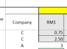
When I enter Company A's 6th entry, for example, A remaining volume is 7. If I enter RM1 consumption N19 value is 3 then Y19 cost should be 3*0.75=2.25
EXCEL_vhW1m3iHmX.png

With the formula you provided, I need the RM1 cost in column N. As per the snapshot above of the Company ABC cost.
 
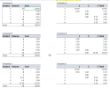
According to the snapshot provided, the costs in the left table and the totals in the right table correspond for Companies A and B. However, there is a discrepancy for Company C. Please verify this.


EXCEL_X0ry81EBX6.png
 
The snapshot below represents the actual company volume and price quantities. Therefore, the final formula to calculate the cost should utilize the company-specific volume, price and Qty's. It means the company input and output are not will be inline, it will be random and mixed. but the condition is N column consumption volume will not be more than the AB column Purchase.

EXCEL_9SAAn97KIa.png
 
The way in which you have presented the problem above requires the formula to filter inputs and output for each company in turn. I have written variants of the MAP function that will then stack the results but that would take you a long way from 'standard' Excel solutions! At present my FIFO calculation does not check the order of input and outputs. It could apply to either the situation in which orders are fulfilled from existing stock or one in which the orders come first and drive custom production. The fulfilment date for each batch would be the order data or the production date, whichever is the later. What is RM2 etc? How do these affect the calculation?
 
If Company A is involved, the entire row of consumption, price, and purchase quantity will only be for Company A, ranging from RM1 to RM10. There will be no clubbing in the same row from RM1 to RM10.

The only consideration is FIFO. We must consume the stock from top to bottom, using the purchases in the order they were entered.
 
A further step.
It would be nice to generate multiple tables with a single formula. That should be possible but uses complex programming techniques.
Code:
= FIFO.SelectedCalc(1, "A", 1)
1729464938675.png
 

Attachments

  • Excel Wizard Solution Chandoo.xlsx
    36.2 KB · Views: 3
@Peter Bartholomew, thank you for your valuable response and the solution you provided. Transferring your solution to my original sheet is proving to be difficult due to its complex programming. I had hoped that someone could adjust the existing formula to use SUMIF or SUMIFS instead of SUM, to manage the sums for each company and calculate the final costs. If it involves VBA coding or an Office script, I could attempt to modify it with AI assistance and apply it to my original file. However, I am uncertain about how to approach the complex programming and where to begin. Additionally, creating tables for each of the 44 companies and 100 RMs presents another challenge with my original file.

Anyway once again thanks a ton for all your efforts @Peter Bartholomew

@all Expecting a simple formula or VBA code to get the results.
 
The formula provided by Copilot AI results in all cells displaying the same value of 0.375. Could someone adjust and provide the corrected formula?

=LET(qty,C4:C18,comp,B4:B18,priceComp,E4:E18,prices,F4:F18,purchaseQty,G4:G18,mPrice,BYROW(comp,LAMBDA(c,IFERROR(INDEX(prices,XMATCH(c,priceComp,0)),0))),mPurchaseQty,BYROW(comp,LAMBDA(c,IFERROR(INDEX(purchaseQty,XMATCH(c,priceComp,0)),0))),usableQty,MIN(qty,mPurchaseQty),usableQty*mPrice)

The sheet is attached here. New simplified version with only RM1.
 

Attachments

  • Cost Sheet.xlsx
    13.3 KB · Views: 3
@Peter Bartholomew, thank you for your valuable response and the solution you provided. Transferring your solution to my original sheet is proving to be difficult due to its complex programming. I had hoped that someone could adjust the existing formula to use SUMIF or SUMIFS instead of SUM, to manage the sums for each company and calculate the final costs. If it involves VBA coding or an Office script, I could attempt to modify it with AI assistance and apply it to my original file. However, I am uncertain about how to approach the complex programming and where to begin. Additionally, creating tables for each of the 44 companies and 100 RMs presents another challenge with my original file.

Anyway once again thanks a ton for all your efforts @Peter Bartholomew

@all Expecting a simple formula or VBA code to get the results.
Firstly, you have posed a complex problem. A basic FIFO calculation is not simple to implement and you require an array of 4,400 FIFO calculations! It may be possible to restrict oneself to the primitive functionality of the traditional spreadsheet and get a solution but I wouldn't be the person to do it! Something that drew my attention to your problem was that I had already written a Lambda function that implemented a FIFO calculation and was intended to be reusable. Filtering would produce results for each company, though doing it 44 times would be a trial.

You might like to take a further look at the solution I am developing to establish whether I have the correct idea of your requirement. So far I have extended the calculation to return a 4x3 array of tables. Getting over the inbuilt array of array limitation introduced by Microsoft's implementation requires even more complex programming than that I have used to date.

I respect your decision not to used the method, after all you need to be confident that you can implement with your real data and maintain it! If you are now looking for a formal code solution, I suggest you repost under VBA macros stating your preferred language (VBA, Python, etc.) using this workbook to explain the requirement. Broadly the level of complexity will be similar whichever language you choose so go for the one you are most familiar with.
 

Attachments

  • FIFO Cost Calculations.xlsx
    39.4 KB · Views: 3
Thank you for your time and effort on my post. If your solution can be easily transferred to my original file, then I must use it. However, my actual file contains many companies and many RMs, so creating a table for each company would be difficult for me. As you suggested, I have already posted this in the VBA Macro section to find a code-based solution.
 
Here is the link to the post in the VBA Macro section for your information.

 
Before moving on, I would like to clear up one apparent misunderstanding. The formula in cell AA34 generates the entire table and could, in theory, be used to generate all 4,400 FIFO result tables within an overall matrix. How that will work out in terms of computational speed, I have no idea. At present, the formula fails if any RM returns a total consumption that exceeds the total purchased. It would be better if the formula were to fail more gracefully with only that particular RM showing an error. Implementation would require copying the formula cell to the new workbook and then ensuring that all the named ranges refer to the correct data objects within your actual workbook.
 
Back
Top