Extracting information between two dates

[Pete Mccann]

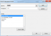
I have a simple question which I am trying to solve with a SUMIFS() formula. Attached is an extract from a Charity database. It contains a list of dates and a quantity of members that joined on particular dates. I would like to create a chart that shows how many members joined in Month X 2017 compared to the number of members joined in the same Month X in 2018. I think I can do the chart but I am struggling with the formula. In cell E11 in the attached I have =SUMIFS(D14:D62,C14:C62,">=e3",C14:C62,"<=e4") [ I know I do not have $ signs added yet]. This formula is intended to calculate "how many people joined in Jan-17, Feb-17 etc." (i.e. between Date E3 and Date E4) but the criteria1 ">=e3" / e4 is not recognised. I can then do a similar calculation for 2018 etc. Any help would be appreciated. If there is another way to plot the data to show, for example, Jan-17 quantity alongside Jan-18 quantities, that would be very useful. The idea is to show how we are progressing in recruiting members into the charity year-on-year.

 

[GraH - Guido]

Something like this, Peter?

 

[Pete Mccann]

Hi Guido - I see you have taken the Pivot Table / Chart route to solve the problem. I tried to do that too but I could not get it to work. I am more familiar with the formula method of constructing the data for the charts. But your solution does indeed answer the question. Is there a formula method too?

 

[Nebu]

Hi:

I still recommend G's method , pivots are designed to summarise data into meaningful information and is much more easier to manage. If you want a formula solution here is one.

Thanks

 

[Pete Mccann]

Thanks guys. I do agree that the Pivot Solution is the better method in this sort of example but I just couldn't seem to get it to work. Also, I had a similar set of formulae in another worksheet and I thought I could tweak it. Thanks again for you replies.

 

[Pete Mccann]

I've been looking at the Pivot solution a bit more. Can you explain how the calculated field is prepared? I would like to show the month-by-month difference (e.g. for each month, what is the difference between 2018-2017). But the calculation is a bit more complicated. To make a fair comparison, there must be a positive value in each month for 2017 and 2018. So, I think it is something like: If Jan 2017 AND Jan 2018 are >0, Difference = (2018-2017). If Jan 2017 OR Jan 2018 =0, Difference = 0. If I try to add a calculated field to do this calculation I get the options as shown in the screenshot. I cannot see how to differentiate the "CountOfDate_Joined" for 2017 from the "CountOfDate_Joined" for 2018. If I can get this field as part of the Pivot chart then I can plot it on the secondary axis.

 

[GraH - Guido]

I used standard pivot features to calculate difference in % of previous

 

[Pete Mccann]

OK, thanks G. I hadn't looked at the Value Field Settings information. Is it possible to put a formula into this area to do the comparison I mentioned earlier? To make a fair comparison, there must be a positive value in each month for 2017 and 2018. So, I think it is something like: If Jan 2017 AND Jan 2018 are >0, Difference = (2018-2017). If Jan 2017 OR Jan 2018 =0, Difference = 0. If I try to add a calculated field to do this calculation I get the options as shown in the screenshot. I cannot see how to differentiate the "CountOfDate_Joined" for 2017 from the "CountOfDate_Joined" for 2018.

 

[GraH - Guido]

One can't enter a formula in the value field settings and in standard pivots I'm not a fan of calculated fields and items. I don't master them neither. I prefer using measures in DAX (power pivot/data model).

But you can do that formula using the same technique as before, @Pete Mccann

Pivot looks like

 

[Pete Mccann]

Thanks G. I think I understand better now what this "value field settings" facility does. It seems quite useful. Best regards.