Kumar Shanmugam
Member
Hi,
I wanted to extract data from a list that match multiple criteria.
I got 75% solution from Luke's post - http://chandoo.org/wp/2014/11/10/formula-forensics-no-003b-lukes-reward-part-ii/
In Luke's post, there is a formula =IF(COUNTIFS($A:$A,$G$6,$B:$B,$G$9,$C:$C,$G$3)<ROWS($I$2:I2),””,INDEX(D:D,SMALL(IF(($A$2:$A$25=$G$6)+($B$2:$B$25=$G$9)+($C$2:$C$25=$G$3)=3,ROW($C$2:$C$25)),ROW(C1))))
I customized the formula for my data: =IF(COUNTIFS(NDCC!$A$1:$A$444,Summary!$A$2,NDCC!$B$1:$B$444,Summary!$B$2)<ROWS($A$10:A10)," ",INDEX(NDCC!$C$1:$C$444,LARGE(IF((NDCC!$A$1:$A$444=Summary!$A$2)+(NDCC!$B$1:$B$444=Summary!$B$2)=2,ROW(NDCC!$B$1:B$444)),ROW(NDCC!C1))))
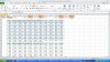
Please refer my sample data:
but criteria is still not completed - I am able to get branches in particular state but i wanted the extracted data to filter in only location having Average buzz greather than state location average and arrear % greater than state arrear.
I am accepting solution like Luke's method.
I wanted to extract data from a list that match multiple criteria.
I got 75% solution from Luke's post - http://chandoo.org/wp/2014/11/10/formula-forensics-no-003b-lukes-reward-part-ii/
In Luke's post, there is a formula =IF(COUNTIFS($A:$A,$G$6,$B:$B,$G$9,$C:$C,$G$3)<ROWS($I$2:I2),””,INDEX(D:D,SMALL(IF(($A$2:$A$25=$G$6)+($B$2:$B$25=$G$9)+($C$2:$C$25=$G$3)=3,ROW($C$2:$C$25)),ROW(C1))))
I customized the formula for my data: =IF(COUNTIFS(NDCC!$A$1:$A$444,Summary!$A$2,NDCC!$B$1:$B$444,Summary!$B$2)<ROWS($A$10:A10)," ",INDEX(NDCC!$C$1:$C$444,LARGE(IF((NDCC!$A$1:$A$444=Summary!$A$2)+(NDCC!$B$1:$B$444=Summary!$B$2)=2,ROW(NDCC!$B$1:B$444)),ROW(NDCC!C1))))
Please refer my sample data:
but criteria is still not completed - I am able to get branches in particular state but i wanted the extracted data to filter in only location having Average buzz greather than state location average and arrear % greater than state arrear.
I am accepting solution like Luke's method.