Excel Filter bug

[Naceur]

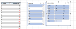
Consider the following 11 Rows x 2 columns table:
LETTERS AMOUNTS
A --------------- 5
B---------------1
C---------------5
D---------------0
A---------------6
B---------------1
C---------------22
D---------------4
A---------------11
B---------------9
Start by filtering out the values "A" and "C" from the LETTERS column.
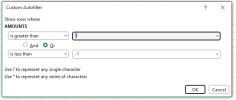
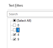
Now, filter out the values 0 and 1 from the AMOUNTS column (you're left with the values 4 and 9)
Now, clear the filter from the LETTERS column.
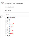
When you check the AMOUNTS column you'll find that all values are filtered out except 4 and 9 (while only the values 0 and 1 should be filtered out)
--------------
When a column is filtered, all values in the other columns should be visible (in the filter drop-down) and it should be possible to select them, even those values that are not "available". The values could be of a grey color but it should always be possible to select them. In the current version, when you apply a filter to a column, the other columns won't show (in the filter drop-down) those values which were filtered out because of a filter in another column.

 

[GraH - Guido]

It's by design, the filtering applies to the range, not a single column.

For problem 1:
When applying the filter on Amounts using this


Works when clearing the first filter.

What you want to see, can be done using values in a table and slicers with the default settings. Show below the value "10" is visible, but the format tells you there are no matching rows, because of the other filter.

 

[Naceur]

Thanks, Grah and Guido, for your replies.

Yes, this works as expected when using Slicers.
However, that approach requires converting the data to a Table, whereas the standard Filter feature itself should behave consistently.

If you refer to the very simple example I gave above (not the larger file with many records), you'll see clearly that the default behavior of Excel Filters does not make sense.

1) Filter out “A” and “C” in the LETTERS column

2) Then filter out “1” and “0” in the AMOUNTS column



Note that the numbers 5, 6, 11 & 22 do not appear (because they correspond to A's and C's, which we already filtered out)

3) Now clear the filter on the LETTERS column — nothing changes.

4) Open the filter dropdown for the AMOUNTS column, and you’ll notice that the values deselected in step 1 (5, 6, 11 & 22 because they correspond to A's and C's) are still deselected.
This shows that filtering out “1” and “0” is effectively treated as “deselect everything, then manually select only 4 and 9”. That explains why those values remain filtered even after clearing the filter on the LETTERS column.



In my view, the standard Excel Filter should behave in the same intuitive way as Slicers, where clearing a filter truly resets the selection context.

 

[Debaser]

The default behaviour does make sense though. As you note, the autofilter list allows you to select the values you want. It is not treated as a list of the values you don't want. The way to specify that (limited to two values) without slicers is to use the custom filter options with 'does not equal'.

If anything, you could argue that the behaviour of slicers is incorrect since they were introduced after the autofilter and should really mirror how autofilters work. As it is, you have an option for working either way, which I would say is better.