• Hi All

    Please note that at the Chandoo.org Forums there is Zero Tolerance to Spam

    Post Spam and you Will Be Deleted as a User

    Hui...

  • When starting a new post, to receive a quicker and more targeted answer, Please include a sample file in the initial post.

Dynamically generate section wise report based on another sheet

jb

Member
Hello helpers,

I have one excel file containing 2 sheets - Data and Report.
Data sheet has multiple rows having date wise tasks performed by one teacher. Each task is included under some heads (section) like exam, activity, seminar etc.
Teacher will keep on adding data in rows date wise.
There can be new heads coming in future.

Teacher needs to generate dynamic report based on data sheet. The report format is given in report sheet. To have an idea, this report is manually typed.
But required to be generated dynamically.

Please help. Sample file attached.
 

Attachments

  • testing.xlsx
    13.7 KB · Views: 15
how about a pivot table
Note your times show 01:30 to 02:30 - so appear by default first as that early in morning/night - should it be PM
that will produce the report and update

what version of excel do you have
 

Attachments

  • testing-ETAF.xlsx
    18.7 KB · Views: 7
hi

check this.. made from power query, you can enter you data entry in data table format.. second sheet just righ click refresh will be updated..
 

Attachments

  • testing1.xlsx
    26.8 KB · Views: 6
how about a pivot table
Note your times show 01:30 to 02:30 - so appear by default first as that early in morning/night - should it be PM
that will produce the report and update

what version of excel do you have
Excel 2010. Also total time of each head is missing
 
Not able to use power query. Any suggestion?

Formula based solution or VBA code is preferred for my problem.
 
Not able to use power query. Formula based solution or VBA code is preferred for my problem
Hello, that must be in the initial post ‼​
According to the initial post attachment a beginner level Excel basics VBA event procedure (v2)​
to paste only to the report worksheet module :​
Code:
Private Sub Worksheet_Activate()
        Dim Rf As Range
        Application.ScreenUpdating = False
        UsedRange.EntireRow.Delete
        [Data!A1].CurrentRegion.Columns("D:I").Copy [A1]
        UsedRange.Sort [F1], 1, Header:=1
        UsedRange.Subtotal 6, xlSum, 4
   With UsedRange.Columns
       .ClearOutline
       .WrapText = False
       .Borders.Weight = 2
       .Cells(.Rows.Count, 4).Borders(8).LineStyle = xlDouble:  .Cells(.Rows.Count, 4).VerticalAlignment = xlBottom
       .Cells(4) = "Time"
       .Item(4).HorizontalAlignment = xlRight:  .Item(4).NumberFormat = " [h]""h""mm "
       .Rows(1).HorizontalAlignment = xlCenter
       .Item("B:C").NumberFormat = " hh:mm "
        Union(.Item(1), .Item("E:F")).NumberFormat = " @ "
        Set Rf = .Item(6).Find("Total *")
   Do
        Rf(1, -4).Resize(, 3).Clear
        Rf(1, -1).Font.Bold = True
        Rf.Cut Rf(1, 0)
        Set Rf = .Item(6).FindNext(Rf(1, 2))
   Loop Until Rf Is Nothing
        Union(.Cells(.Rows.Count, 5), .Item(6)).Clear
       .AutoFit
   End With
        Application.ScreenUpdating = True
End Sub
Do you like it ? So thanks to click on bottom right Like !​
 
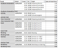
Or a plain pivot:

1718818012267.png

I've converted the data sheet to a proper table so that when new data is added it will expand automatically.
The pivot will need refreshing if the source data on the data sheet changes; right-click on the pivot and chose Refresh (or this could be done automatically).

Edit after posting: Just saw that @ETAF proposed very similar, however I have included subtotals for the Head
 

Attachments

  • Chandoo57159testing.xlsx
    25.3 KB · Views: 5
Or a plain pivot:

View attachment 87485

I've converted the data sheet to a proper table so that when new data is added it will expand automatically.
The pivot will need refreshing if the source data on the data sheet changes; right-click on the pivot and chose Refresh (or this could be done automatically).

Edit after posting: Just saw that @ETAF proposed very similar, however I have included subtotals for the Head
I explored the method of creating pivot table and I tried creating pivot table but I am not getting format like you have created.

First, when I add head column in pivot table it shows the column label as "Row labels".

Next when I add the column date2, from, to and topic, it shows them in the same column of head one after another.

I am not able to understand where I am doing mistake. Can you explain the correct process?

Please look at my file where I have tried to create pivot table.
 

Attachments

  • Chandoo57159testing.xlsx
    24.8 KB · Views: 1
1. Put the selection somewhere in your new pivot, then on the Design tab, Layout section, Report Layout, choose Show in Tabular Form

1720216287814.png

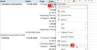
2. Your Excel sems to have automatically grouped the To and From fields, so they need to be ungrouped:
Right-click a value in the From field and choose ungroup. Do the same for the To field.
1720216455383.png


3. There is too much sub-totalling going on so again in the Design tab, choose Do not Show Subtotals:

1720216643298.png

This removes all subtotalling but we want to keep it for the Head field, so right-click somthing in the Head field and choose Subtotal Head:

1720216780741.png

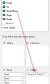
Now add Total Time field to the Values area:

1720216938186.png

Mine defaulted to Count of total time, we need to change that to Sum of Total Time.
See next message (only allowed to add 5 pics per message).
 
Last edited:
Click on the down arrow (yellow blob below) and choose Value field settings…

1720217098428.png

then in the dialogue box choose Sum:

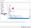
1720217345144.png

but before we click OK on this dialogue box, we'll click on Number Format and change the format to [h]:mm (type it in if it's not in the list):

1720217477220.png
Then click OK on these dialogues.

After all that you can tart it up as you want; choose a different Pivot table style, remove the +- boxes, change the headers etc.
 

Attachments

  • 1720217225346.png
    1720217225346.png
    15.1 KB · Views: 1
Last edited:
  • Like
Reactions: jb
Click on the down arrow (yellow blob below) and choose Value field settings…

View attachment 87570

then in the dialogue box choose Sum:

View attachment 87572

but before we click OK on this dialogue box, we'll click on Number Format and change the format to [h]:mm (type it in if it's not in the list):

View attachment 87573
Then click OK on these dialogues.

After all that you can tart it up as you want; choose a different Pivot table style, remove the +- boxes, change the headers etc.

Thank you for your help. I followed your steps. Everything works fine but when I am adding from and to column, it is not preserving the format in which I have entered the data. It attach AM or PM with time. Kindly suggest how to preserve time format as per original data in pivot table.

Also it adds one column with title Hours2 between From and To column. Can you please explain this behaviour? Also suggest how to avoid this extra column. Thank you in advance.
 

Attachments

  • Chandoo57159testing.xlsx
    27.4 KB · Views: 1
Also it adds one column with title Hours2 between From and To column. Can you please explain this behaviour?
It's the grouping it does for you automatically - a pain. You'll need to ungroup again, as mentioned in step 2. There may be a setting somewhere to prevent it being 'helpful'!
It attach AM or PM with time. Kindly suggest how to preserve time format as per original data in pivot table.
You'll need to go into Number format in Field settings to reset the formatting.
 
Last edited:
  • Like
Reactions: jb
It's the grouping it does for you automatically - a pain. You'll need to ungroup again, as mentioned in step 2. There may be a setting somewhere to prevent it being 'helpful'!

You'll need to go into Number format in Field settings to reset the formatting.

Sir, I copied pivot table suggested by p45cal and applied on my actual data. Last column is sum of total time column. It gives wired answer for some rows. Say for example, 17-06-2024 - 9:40 to 10:30 it gives 00:50 which is correct.
But for 24-06-2024, 27-06-2024, 28-06-2024 and 01-07-2024 - 9:40 to 10:30 it gives 01:40 which is incorrect.
This happens for 25-06-2024 - 11:30 to 12:20 - it should give 00:50 but giving 01:40.
How this happened?

1720412972068.png
 
According to your guessing challenge check the source data are numeric rather than text unlike your 'dates' in your initial post attachment …​
 
According to your guessing challenge check the source data are numeric rather than text unlike your 'dates' in your initial post attachment …​
Sir, total time column is based on subtraction of To minus From column. And I checked the format. It is not text. It is in hh:mm format. In the data sheet, it calculates the time difference correctly. But in pivot table for few entries correct answer showing and for few entries wrong answer.

I am attaching my original file here.
 

Attachments

  • testing2.xlsx
    83.4 KB · Views: 3
Last edited:
It's the sum of all lines in your source data that match; for example, for
25-06-2024 the pivot shows:
1720441330343.png

because 2 lines from your data fulfil the Head (Session), Date_R (25-06-2024), From (9:40), To (10:30), Topic (both exactly the same), so both rows' time of 50mins are summed (=1:40).

1720441262183.png

If you see unexpected results like this, you can double-click on the result (1:40 in the Sum of Total Time column), and Excel will create a new sheet showing the rows of data in the source that have been used to get the result you double-clicked on. It looks like this:

1720441706012.png

You can delete the sheet after viewing it.

If you want to see these as separate rows in the pivot, include another field in the pivot that has different values, such as the Class field or the Subject Code.
 
Last edited:
It's the sum of all lines in your source data that match; for example, for
25-06-2024 the pivot shows:
View attachment 87597

because 2 lines from your data fulfil the Head (Session), Date_R (25-06-2024), From (9:40), To (10:30), Topic (both exactly the same), so both rows' time of 50mins are summed (=1:40).

View attachment 87596

If you see unexpected results like this, you can double-click on the result (1:40 in the Sum of Total Time column), and Excel will create a new sheet showing the rows of data in the source that have been used to get the result you double-clicked on. It looks like this:

View attachment 87598

You can delete the sheet after viewing it.

If you want to see these as separate rows in the pivot, include another field in the pivot that has different values, such as the Class field or the Subject Code.
It worked. Thank you so much sir for your help and explanation. Thank you again.
 
Back
Top