• Hi All

    Please note that at the Chandoo.org Forums there is Zero Tolerance to Spam

    Post Spam and you Will Be Deleted as a User

    Hui...

  • When starting a new post, to receive a quicker and more targeted answer, Please include a sample file in the initial post.

Correct Excel formula

subhi

New Member
In the attached sheet....... the cells B2,D2,F2,H2 are IDs and some of them have the same ID "FON", and the cells A2,C2,E3,G3 are the names of those IDs.

I need an excel formula to find the name which matchs the first ID "FON" which will be applied in cell L1 also the name which matchs the second ID "FON " which will be applied in cell N1, and the same thing for the name which maths the third ID "FON " which will be applied in cell P1.
 

Attachments

  • Formula1.csv
    127 bytes · Views: 16

subhi

Your 'sheet' looks like below ...
Screenshot 2024-02-14 at 19.26.00.png
Where would You expect to need ... an Excel formula?
What would be Your expected results?
Do You always have there two lines data?
 

subhi

Your 'sheet' looks like below ...
View attachment 86460
Where would You expect to need ... an Excel formula?
What would be Your expected results?
Do You always have there two lines data?

You can see the attached sheet.

the answers as below in cells (L2,N2 and P2):
1707939614516.png

Yes, the two data lines always there.
 

Attachments

  • Formula.xlsx
    8.8 KB · Views: 4
As asked:
What would be Your expected results?
Your the answers as below in cells (L2,N2 and P2):
... which are empty!
 
There seems to be something wilfully perverse about the alternating arrangement of the data and associated results!
That said
Code:
= LET(
    wrapped, WRAPROWS(data, 2),
    matches, FILTER(TAKE(wrapped,,1), TAKE(wrapped,,-1) = "FON"),
    TOROW(HSTACK("Result " & SEQUENCE(ROWS(matches)), matches))
  )
will return the result described for a single row of data.
 
In L1:
=IFERROR(INDEX(FILTER($A2:$G2,$B2:$H2="FON"),1),"")
In N1:
=IFERROR(INDEX(FILTER($A2:$G2,$B2:$H2="FON"),2),"")
In P1:
=IFERROR(INDEX(FILTER($A2:$G2,$B2:$H2="FON"),3),"")

Can copy down.
 
I need the formulas which acheive the below :

Cell L1 : looking for the First cell which have "FON" from the range ( A2:H2) and take the name before it which will be "C1335".
Cell N1 : looking for the Second cell which have "FON" from the range ( A2:H2) and take the name before it which will be "C1279".
Cell P1 : looking for the Third cell which have "FON" from the range ( A2:H2) and take the name before it which will be "C1409".
 
There seems to be something wilfully perverse about the alternating arrangement of the data and associated results!
That said
Code:
= LET(
    wrapped, WRAPROWS(data, 2),
    matches, FILTER(TAKE(wrapped,,1), TAKE(wrapped,,-1) = "FON"),
    TOROW(HSTACK("Result " & SEQUENCE(ROWS(matches)), matches))
  )
will return the result described for a single row of data

I need to apply this command using excel formula, Could you help me please.
 
What is missing?
Do You have own formula?
To make it easy and clear for you.
Based on the attach sheet, I need the excel formula which will be applied in cells (P1,R1 and T1) which gives the result after looking on the range of cells (A2:J2) and the first cell which contains "FON" I need to take the value of the cell before it and but it in the cell P1, then that looking on the range of cells (A2:J2) and the second cell which contains "FON" I need to take the value of the cell before it and but it in the cell R1, then that looking on the range of cells (A2:J2) and the third cell which contains "FON" I need to take the value of the cell before it and but it in the cell T1.......the correct answer is ( P1= C1335 , R1= C1279 , T1= C1388).
 

Attachments

  • Formula.xlsx
    8.9 KB · Views: 1
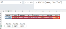
Not quite the output format you request but with 2021 you could use the trick of offset defined ranges along with FILTER.
1709767526412.png
 

Attachments

  • Formula (1).xlsx
    17.2 KB · Views: 3

subhi

Your To make it easy and clear for you.
Your original thread was
the cells B2,D2,F2,H2 are IDs and some of them have the same ID "FON", and the cells A2,C2,E3,G3 are the names of those IDs.
Three FONs from four pairs and results starts from cell K1.
Your newer file has different number or pairs and results starts from different cell.
Should I or someone guess - what next?

subhi

Yes, reply #20 could be a solution, if You'll accept other layout of results.
 
Last edited:

subhi

Your To make it easy and clear for you.
Your original thread was
the cells B2,D2,F2,H2 are IDs and some of them have the same ID "FON", and the cells A2,C2,E3,G3 are the names of those IDs.
Three FONs from four pairs and results starts from cell K1.
Your newer file has different number or pairs and results starts from different cell.
Should I or someone guess - what next?
No worries, the sheet which shared by Mr. Peter is working fine.
Thanks for your support.
 
Back
Top