Hi ,
You are right that using AND did not work , but the reason is different.
Conditional Formatting is applied by selecting a range and then defining the rules which will be applied to the range for deciding on the format to be applied.
However , when you define the rule , the principle is that the rule uses the top left hand corner cell of the selected range ; thus if your range of data is B1 through B17 , you will first select this range and then use the formula :
=AND(B1 <> "" , B1 < 0.6 )
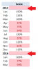
You have used A1 , but the screenshot you have uploaded clearly shows a column of data to the left of the column which has the percentages to be tested. Hence I have assumed that the column to be used in the formula should be column B , rather than column A. If this is also incorrect , you will need to correct the above formula.
Secondly , the usage of the $ sign should be well-thought out.
Using the $ sign and making the formula :
=AND($B$1 <> "" , $B$1 < 0.6 )
means that all the cells in the selected range will be colored based on the checking of only B1.
Without the $ sign , Excel will look at cell B1 for coloring B1 , cell B2 for coloring B2 , cell B3 for coloring B3 and so on.
If you use the $ sign in front of the column reference , as in :
=AND($B1 <> "" , $B1 < 0.6 )
it will not make any difference if you have selected only the range B1:B17 ; however , if you select the range A1:B17 , then the above formula will ensure that cells in both columns will be colored based on the values in column B.
Narayan