• Hi All

    Please note that at the Chandoo.org Forums there is Zero Tolerance to Spam

    Post Spam and you Will Be Deleted as a User

    Hui...

  • When starting a new post, to receive a quicker and more targeted answer, Please include a sample file in the initial post.

Conditional Formatting Help

jwaltz

New Member
1724722020491.png
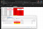
Row K shows the last time a child was seen.

Row L shows the last time a child was seen unannounced.

I need Row M to reflect the color Orange in 15 days from the date information in Row K.

I need Row M to reflect the color Red in 20 days from the date information in Row K.

I need Row N to reflect the color Orange in 80 days from the date information in Row L.

I need Row N to reflect the color Red in 90 days from the date information in Row L.


I have attempted using Conditional Formatting and I cannot figure out the formula.


Can someone please help?
 
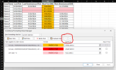
Select M2 - click on Conditional Formatting on the ribbon - you will now be able to see three CF rules.
 
Yep! The formulas must be created similarly to the way you did for the = 0 pink format.
For each Cell that the "Conditional" format has been applied, you will find the formulas for that Cell only by reviewing the Rules applied to the Cell.

So if you want to see the formulas for Column N, you would select a cell in that column and review the rules. If you need to extend the formatting to other cells you may copy and paste the format or the entire cell.

Play with the order of the Rules too, it matters as they run from the top of the rules to the bottom unless you check the "Stop if True" box for one.

1724856267170.png
 
The basic formula that I've used is:
=IFERROR(IF(AND(NOT(ISBLANK(K2)), M2 >= (K2+15)),TRUE,FALSE),FALSE)

I added columns to your file that have no other purpose than to demonstrate the formulas. Keep in mind that the CF rules run one after the other and the last one wins or overwrites the last if the value evaluates to "True".

Let us know if you have any other questions.

Cheers!


Attachments

  • Sample.xlsx
    10.9 KB · Views: 3
Okay, so I'm going insane. I love all of this help but there has got to be something wrong with me and what I am doing. (In my spreadsheet I need it for) In Column M, as soon as I put in the conditional formatting for the red, everything turns red, which it should, because now all kiddos are on or after day 20. However, when I put in the conditional formatting for the orange, everything turns orange.

I'm going to cry lol.
 

Attachments

  • Sample (2).xlsx
    10.5 KB · Views: 4
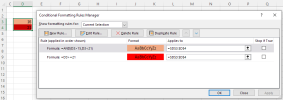
PLEASE don't cry. It is indeed MY fault. I hadn't tested the "Stop if True" check box and assumed it operated as it suggests by its existence. Unfortunately, CF seems to ignore the check and treats all lines as if all the boxes are checked.

Just look back at the order I posted in Post 7. Then use your arrows to ensure you are using the correct order.

Orange is always true if Red is true to agree with your needs. So the rules are stopping there. Move Red up and you'll be fine.

1724863308557.png
 
@ExcelGoogler
=IFERROR(IF(AND(NOT(ISBLANK(K2)), M2 >= (K2+15)),TRUE,FALSE),FALSE)
is unnecessarily complicated for CF in this case. Various functions like IF, FALSE TRUE are implicit (as are array formulas in CF)
e.g.
Code:
=AND($B2>0;$D2>0;$D2>$B2+15;$D2<=$B2+20)
is more than enough
@jwaltz
I added CF to col D ( see attached) . I trust you will be able to build the CF for col E based on the attached if it fits your needs. However you did not say what should happen when dates are larger than +20 or +90 ?
 

Attachments

  • Sample(10).xlsx
    11.1 KB · Views: 3
I hadn't tested the "Stop if True" check box and assumed it operated as it suggests by its existence. Unfortunately, CF seems to ignore the check and treats all lines as if all the boxes are checked.
Yes, conditional formatting is very confusing indeed. When I had a look at this I thought it wasn't working as it should and Stop if True seemed a bit random!
So looking into it a bit deeper I found where I was going wrong.

The first thing I noted was that the first of the conditional formats that was TRUE was king and even if conditional formatting lower down the list was also TRUE, that lower down CF did not apply if the formatting was in conflict with the first that was true.
It's that last underlined bit which is important.
When you go into setting the formatting from the conditional formatting dialogue box, there are several aspects of formatting which you can change. Importantly, there are aspects which are not 'set' in a given CF. Those 'unset' aspects do not change the formatting that was there before.
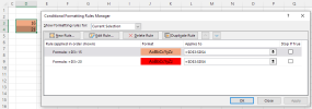
Here's a pic:
1725224856889.png

You can see above that one cell fulfils the 2nd CF and both cells fulfil the first, but only the top CF is in action, because the aspect that each CF is trying to affect is the fill colour of the cell. (An easy way to rectify this in this case is to reverse the order of CFs.)
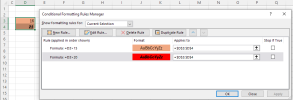
To show you that the second CF is actually in operation I'll set some more aspects of formatting for the 2nd CF (bold italic and strike-through):
1725225346546.png

Where you can see that those aspects have been applied to cell D4 only, but that the brown of the first CF remains and the red doesn't show at all.

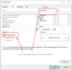
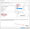
When setting the CF you get a Clear button. This what you see before clicking it:
1725225612790.png

and after clicking it:

1725225826605.png

So if a true CF has an aspect of formatting that is in conflict with another true one higher up it doesn't show; if it's not in conflict it will show.

Finally, Stop if True works as expected, here you can see that the 2nd CF hasn't been applied at all:

1725226117221.png


So while not giving you the actual CFs you want (there are several questions that I'd need answering before doing that) I hope I've equipped you with what's necessary to stop you going insane!

(I've not come across this sort of stuff on the interweb much at all; most of this is through trial and error.)
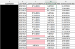
continued in next message; can only add 5 pictures…
 
Last edited:
…continued from above.
Apart from putting the CFs in an appropriate order to ensure you get the CF appearance you want, if that ends up being difficult you can also change the formula to make CF rules 'exclusive'. Here the CFs can be in any order:

1725227649359.png
 
Back
Top