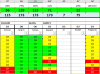
in the above sheet values in A2:D6 will be either (NP, D2, D3 or OK). How to get automatically with formula to return a text in say column E2. Check cells (A2:D2) Condition1 is if any of the cell value is "NP" the value to be returned in is "NP". Condition2 if no "NP" then if there is D2 it should return D2. If none of the cells are with "NP" & "D2" if it has "D3" then return "D3". If all cells is with ÖK" then value to be returned is OK.
You are using an out of date browser. It may not display this or other websites correctly.
You should upgrade or use an alternative browser.
You should upgrade or use an alternative browser.
CHECK TEXT IN DIFFERENT CELLS AND RETURN VALUE IN ANOTHER CELL
- Thread starter Pugazh
- Start date
Pugazh
Please reread:
https://chandoo.org/forum/threads/site-rules-new-users-please-read.294/
Please Don't ... the 1st sentence
=IF(COUNTIF(A2:D2,"OK")=4,"OK",IF(COUNTIF(A2:D2,"NP")>0,"NP",IF(COUNTIF(A2:D2,"D2"),"D2","D3")))
or
Did You really mean ...
If none of the cells are with "NP" & "D2" if it has "D3" then return "D3".
then how next sentence can be possible?
If all cells is with ÖK" then value to be returned is OK.
Last edited:
1] How does =SUBTOTAL(103,E2:E3) return value as 5 ? Only 2 cells in E2:E3, should return 2.Dear Bosco,
Thanks. This works but i am not able to do subtotal of all the values returned. Means subtotal(103,E2:E3) = is showing blank. it should return value as 5.
2] Please forward us more information as well as a sample file.
Regards
Bosco
1] I don’t know why Subtotal can't work in Column G?
2] I try to use a helper column. In H2, enter: =G2, and copied down to H6
3] In H1, enter: =SUBTOTAL(103,H2:H6), and it is working when filter is applied.
4] Maybe someone can help to give you an answer
5] Sorry in unable to help.
Regards
Bosco
2] I try to use a helper column. In H2, enter: =G2, and copied down to H6
3] In H1, enter: =SUBTOTAL(103,H2:H6), and it is working when filter is applied.
4] Maybe someone can help to give you an answer
5] Sorry in unable to help.
Regards
Bosco
Last edited:

Dear Bosco,
Subtotal returning null value is solved by using formula with Sumproduct/subtotal/offset formula.
can you help in solving - if there is no entry or value in cells A7:F7 it returns #NUM!. cell G7 should be blank. Formula in cell G7 is =INDEX({"NP";"D2";"D3";"OK";""},AGGREGATE(15,6,MATCH(A7:F7,{"NP";"D2";"D3";"OK";""},0),1))
Try,Dear Bosco,
Subtotal returning null value is solved by using formula with Sumproduct/subtotal/offset formula.
can you help in solving - if there is no entry or value in cells A7:F7 it returns #NUM!. cell G7 should be blank. Formula in cell G7 is =INDEX({"NP";"D2";"D3";"OK";""},AGGREGATE(15,6,MATCH(A7:F7,{"NP";"D2";"D3";"OK";""},0),1))
View attachment 57640
=IF(COUNTA(A2:F2),INDEX({"NP";"D2";"D3";"OK"},AGGREGATE(15,6,MATCH(A2:F2,{"NP";"D2";"D3";"OK"},0),1)),"")
Regards
Bosco