• Hi All

    Please note that at the Chandoo.org Forums there is Zero Tolerance to Spam

    Post Spam and you Will Be Deleted as a User

    Hui...

  • When starting a new post, to receive a quicker and more targeted answer, Please include a sample file in the initial post.

I want to color code certain cells based on 2 to 6 vertical cells

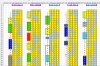
I want to be able to color code cells in a column based upon certain criteria. For example, if I have the numbers 2-4-6 vertically I want to color code them yellow with blue font and a blue border. If someone can show me how o do 1 I can o the rest. I have several columns with 3000 rows in each that I will be coding

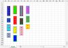
In the example you can see in AE:8 through AE:10 or AS:13 - AS:15. I have the 246 color coded. I want to be able to color code all the 246 on a sheet but I do not want to capture every 2,4,6. Only the ones in a vertical row. Another example would be the 6622 in AE:11 - AE:14 or AL:10 through AL:13.

How can I write the conditional formatting to do this?

Thanks Guru's
 

Attachments

  • Pattern and CF Chando.jpg
    Pattern and CF Chando.jpg
    306.7 KB · Views: 16
Hi Jack -
I think you can do the following - I did not try it though..

Go to conditional formatting - Use a formula to determine which cells to format..and use the AND function..

This should work i guess
 
Hi Larry ,

See the attached file , and note the range over which the rules have been applied , and the 3 rules ; when you implement this on your file , you will have to change these appropriately. If your data starts on rows 1 or 2 , you will need to change the applied ranges also , since for the third rule you cannot refer to a row which is 2 rows above it.

Narayan
 

Attachments

  • Example.xlsx
    10 KB · Views: 7
Hi Larry ,

See the attached file , and note the range over which the rules have been applied , and the 3 rules ; when you implement this on your file , you will have to change these appropriately. If your data starts on rows 1 or 2 , you will need to change the applied ranges also , since for the third rule you cannot refer to a row which is 2 rows above it.

Narayan

Excellent as always Narayan, how do I do ones with only 2 numbers like 6-8 or 4 numbers like 8-2-4-6, what needs to be changed
 
Hi Larry ,

The philosophy is straightforward :

1. If you have 'x' number of cells which form a sequence that you wish to format , then if 'x' equals 2 , you need to have 2 rules ; in each rule , you will look at the current cell , and either the cell below that cell if it is the upper cell , or the cell above that cell if it is the lower cell ; I hope that is not too confusing !

In your present case , there are 3 cells which form a sequence , and so 3 rules are required ; the upper-most cell looks at its own value to be equal to 6 , and the next one below it to be equal to 4 , and the one below that to be equal to 2 , thus forming a sequence 6 , 4 , 2. The middle row cell will have to look at the cell above it being equal to 6 , its own value being 4 , and the cell below it having 2. The lower-most cell will have to look for the two cells above it having the values 6 and 4 , while its own value should equal 2.

So , if you have a sequence of 4 cells , you will need to have 4 rules ; suppose your range is A4 through A1000 ; the rules will be :

=AND(A4=8 , A5=2 , A6=4 , A7=6)

=AND(A3=8 , A4=2 , A5=4 , A6=6)

=AND(A2=8 , A3=2 , A4=4 , A5=6)

=AND(A1=8 , A2=2 , A3=4 , A4=6)

Select the range A4:A1000 and apply the above 4 rules.

If your data starts from rows 1 , 2 or 3 , you will need to change the rules and range to which the rules are applied.

There will probably be one single array formula which can look at the desired number of cells and see whether that contain the desired sequence , but this is a simple technique , and only if you cannot implement this should we look for an alternative.

Narayan
 
Hi Larry ,

You are right , but you also have to select the range A3 through say A1000 when you apply these rules. If the range selected starts from A2 or A4 or any other cell in column A , then your rules will need to have their references changed. The rules you have posted will work only if the range selected to apply them is A3 through any other cell in column A below row 3.

Narayan
 
Thanks again, I will give it try

Do I highlight only say 2 cells if I am using 2 cells like A1 and A2 or does it not matter as long as I am on A?
 
Hi Larry ,

You need to select the data range where you want this CF to be applied ; if that is just 2 cells , then it has to be as follows :

If you select A2 and A3 , then your 2 rules will refer to :

1. A2 and A3 - the first cell in the selected range , and the cell below it
2. A1 and A2 - the first cell in the selected range , and the cell above it

If you select A3 and A4 , then your 2 rules will refer to :

1. A3 and A4 - the first cell in the selected range , and the cell below it
2. A2 and A3 - the first cell in the selected range , and the cell above it

If you select A4 and A5 , then your 2 rules will refer to :

1. A4 and A5 - the first cell in the selected range , and the cell below it
2. A3 and A4 - the first cell in the selected range , and the cell above it

If you select A5 and A6 , then your 2 rules will refer to :

1. A5 and A6 - the first cell in the selected range , and the cell below it
2. A4 and A5 - the first cell in the selected range , and the cell above it

You get the drift ?

Narayan
Yes I get your drift. What's confusing is I can high lite A1:A3 and it will color code ALL the ones in the column. I've always thought you had to high lite the entire column to catch all involved.

Okay, 1 more question I hope lol) once I program 1 column with all the CF I want how do I copy just the formatting to all the other columns? I've tried different paste options and can't seem to find the correct one I've been using the icon that has a percentage symbol and a paint brush but sometimes it works and sometimes it doesn't

Hmmm, wish I knew how to do a Macro for these, seems like it would be easier but then again idk. I only have maybe 8 to 12 different sets I color code and using conditional formatting I have to rewrite every one individually.
 
Hi Larry ,

If you select the range A1:A3 and then enter the CF rules , it cannot highlight all sequences in the entire column ; Excel does not work that way.

I suggest you clear all CF rules in the column and then select A1:A3 , and then set up the rules.

However , as I have mentioned earlier , if you have two rules , if your data starts from A1 , the procedure will be different.

Can you specify :

a. What is your data range over which you want to apply the CF rules ?

b. What is the sequence you wish to check for ? Is it 2 numbers , or 3 or 4 ?

Narayan
 
I agree, it should not work like that but it is. LOL. I will do as you suggest but i already did that last night because it made no sense but then again I have seen office 2013 do some weird things that 2010 do not
okay , let me give you my complete picture perhaps this is more than I thought it would be.

Here are the main patterns I look fr and any of these can be in any of the columns and rows

Again, thank you for all your help!!!
 

Attachments

  • Patterns I use.xlsx
    9.7 KB · Views: 2
  • Patterns.xlsx.jpg
    Patterns.xlsx.jpg
    96.1 KB · Views: 6
Hi Larry ,

Can you upload at least one data file where you want to implement the CF rules for these sequences ?

Narayan
 
Hi Larry ,

See your file ; I have introduced only one pattern's rules ( 3 in this case ) for the pattern 6 - 4 - 2. This has been done in column B ; since only relative addressing has been used , you can copy this format to all other relevant columns and it will work correctly.

You have a total of 14 patterns involving a total of 47 rules ; this is a lot of work.

Narayan
 

Attachments

  • Numbers Patterns Nar.xlsx
    116.9 KB · Views: 3
Thanks Narayan!

I don't mind doing the work because this is one of 18 sheets in 1 out of 5 books that changes every 7 to 10 weeks. So, once I gave the CF completed it will do the color coding automatically (-:

Which paste option us best to use to copy the formatting? I've been using the one with the paint brush
 
Hi Larry ,

That is the one ; it's called Format Painter , and you can certainly use it.

Narayan

Thanks!! If you noticed on the sheet I uploaded the 8 in Column R will not allow shading to change or go away. No clue why. I was trying to code the 86 and when I even clear the rule it stays shaded
 
Hi Larry ,

Please remember that the other columns may all have some CF rules already ; if you are going to copy the format from column B , select the other columns where you will be copying the format , clear the conditional formats from those selected columns , and thereafter copy the format from column B to those columns. Otherwise what ever formats are present in column B will be added to the formats already present in those columns.

Narayan
 
This is what is driving me crazy, I used the following rules to make the same column using the same numbers 246 BUT they go the other direction which should not matter and I can not seem to get it right. What am I missing please Narayan?

=AND(B7=2,B8=4,B9=6) =$B$7:$B$66

=AND(B6=2,B7=4,B8=6) =$B$7:$B$66

=AND(B5=2,B6=4,B7=6) =$B$7:$B$66
 

Attachments

  • NarOB.xlsx
    113.2 KB · Views: 1
Hi Larry ,

Please remember that the other columns may all have some CF rules already ; if you are going to copy the format from column B , select the other columns where you will be copying the format , clear the conditional formats from those selected columns , and thereafter copy the format from column B to those columns. Otherwise what ever formats are present in column B will be added to the formats already present in those columns.

Narayan


Yes sir, I understand. I am going to program 1 column with all the formatting and then clear all the others and then do the copy and paste.

Naratan, THANK YOU so much for your patience. I have learned so much from you and try my best not to bother you unless I need to. I REALLY want to learn this
 
Hi Larry ,

The problem with having 2 sequences is that you have to decide what is to be done in a case where you have both sequences overlapping ; for instance , suppose you have the following sequence of numbers from the top down :

2
4
6
4
2

The 2 , 4 , 6 form one sequence which needs to be colored one way ; the 6 , 4 , 2 form another sequence which needs to be colored a different way.

If you do not do anything , then you will have partial coloring where only 2 numbers in the sequence are colored even though you can see that the three numbers are in sequence , since the 2 , 4 will be colored one way , while the 6 , 4 , 2 will be colored the other way.

What is to be done in this case ?

Narayan

It really does not matter to me as ling as they are colored. When I am looking at 3000 rows it sticks out. So for arguments sake pick either overlap to be one of the same colors OR if possible make the overlap red so I know it is an overlap (and I just thought about this)
 
I do use the SAME number sequence for all patterns correct?? (=AND(B7=6,B8=4,B9=2) Just change the pattern (642 to 2266) and of course add the other (4th) rule for this one

=AND(B7=6,B8=4,B9=2) =$B$7:$B$66

=AND(B6=6,B7=4,B8=2) =$B$7:$B$66

=AND(B5=6,B6=4,B7=2) =$B$7:$B$66
 
Back
Top