HOWTO: Calculate how many business days for the following sample data ? Additional explanation provided.

[AGYANI]

Dear Excel_Lence Gurus !

I humbly ask for your help and guidance in the challenge I am facing, and trying to see how I can automate or a logic for calculating few performance metrics in days , given few dates and no. of quality control checks made on a application.

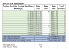
The out put is shown in the table e.g APPLICATION # 2023-02030 If you notice the first time the application was inserted to be tracked was on Feb 10 2023 and the first time a QA person looked at it was on April 02 2023, So the number of business days elapsed =NETWORKDAYS.INTL(G3,H3) = 36 days on April 2 2023 the QA person saw 3 defects and subsequently on the same day additional defects were found e.g 4,2,0,2,2,2.

APPLICATION # 2023-02030 stayed in the weekly excel file from Feb 10 2023 thru Sept 10 2023 , when the second QA check on May 1 2023, that is about 21 business days elapsed since the first time on April 4 2023 , and on May 1 2023 there were additional 3 more defects found and additional 4,3,4 defects throughout that day and the last Check was performed on May 24th 2023 by the QA person and additional 3 defects were found. If you notice the APPLICATION # 2023-02030 was all thru tracked from Feb 10 2023 thru Oct 23 2023 in Column G

The metrics I am trying to calculate: For APPLICATION # 2023-02030
Total Days with the applicant = 75 Business days [10 weeks 5 days] =SUM(I4:I14)+ABS(I3) #

Days Project[Application #] tracked = 182 days [26 weeks] =NETWORKDAYS.INTL(G3,G14)
Last time QA tracked since first time it was tracked =74 days[10 weeks 4 days]==NETWORKDAYS.INTL(G3,H14)



Important Note: The dates in column G and H have to be sorted by Ascending order as the time moves only forward. In the raw data , please make sure for each Application # , this is consistent and Column J : Is redundant , as it is the same as COlumn H, also reason I am taking the ABS(I3) value is because sometime the QA check is completed before the tracking starts.

Output Requirement: If this data can be tabulated in form of a excel Sheet with instead of the way it is presented with the following information for the 510 application over 69 weeks.

Column-A : Application #
Column- B :Total Days with the applicant
Column-C :Days Project[Application#] tracked
Column-D: Last time QA tracked since first time it was tracked



My excel sheet has the following column headers:

Tracked Excel File Created Date[Every Mondays]	Application# is tracked in this file from the start date[When the application was first checked and stays in the subsequent file till it is dropped off]	Date Format
Application#	Application #	Format YYYY-#####
Date Last Checked	This field contains the Date when a "Check" were performed by QA expert	Date Format
Checks	This is the number of Deficiency found	Number [Integer]

 

[Monty]

Hello Agyani

Here's a basic outline of the formulas you might use:Column B (Total Days with the applicant):

=SUM(I4:I14)+ABS(I3)

Column C (Days Project[Application#] tracked):=NETWORKDAYS.INTL(G3,G14)Column D (Last time QA tracked since first time it was tracked):

=NETWORKDAYS.INTL(G3,H14)

You can apply these formulas to each row for the corresponding application.Regarding the output requirement for the Excel sheet, you can create a new sheet and structure it with the specified columns:

Column A: Application # Column B: Total Days with the applicant
Column C: Days Project[Application#] tracked Column D: Last time QA tracked since first time it was tracked

 

[AGYANI]

@Monty Thank you for quick response, We have to group it by Application# as application same application can exist in many tracking excel file. as you notice, as I said there are only 510 Applications# over 69 weeks of data, the raw data is in the "Sample.xlsx" file and the picture is how I am calculating each Application #,

 

[Monty]

In that case the data by Application # and calculate the metrics for each unique application, you can use Excel's PivotTable feature. Here's a step-by-step guide:

1. Open your "Sample.xlsx" file.

2. Select the range of your data, including column headers.

3. Go to the "Insert" tab in the Excel ribbon and click on "PivotTable."

4. In the PivotTable dialog box, ensure that the "Select a table or range" field points to your data range. Choose where you want to place the PivotTable (e.g., a new worksheet), and click "OK."

5. In the PivotTable Fields pane, drag the "Application#" field to the Rows area.

6. Drag the "Total Days with the applicant," "Days Project[Application#] tracked," and "Last time QA tracked since first time it was tracked" fields to the Values area. Ensure that these fields are set to calculate as needed (e.g., sum or average).

7. You should now have a PivotTable with Application # in the rows and the calculated metrics in the values.

8. To make it more presentable, you can format the PivotTable and adjust the column headers as needed.

This PivotTable will give you a grouped view of the metrics for each Application # over the specified weeks.

 

[AGYANI]

@Monty Thank you, the pivot method does not solve my question, I need to calculate "business day" count based on the calculated field of the Tracked Excel File Created Date[Every Mondays] and " Date Last Checked", if you look at the image I have attached "Days with Applicant" is calculated when there is c change in the "Date Last Checked". If you notice the first number 36 days is calculated by =NETWORKDAYS.INTL(G3,H3) = 36 days and the subsequent value of 21 days is calculated by subtracting NETWORKDAYS.INTL(H9,H10)= 21 and the next value NETWORKDAYS.INTL(H13,H14)= 18

So total days with applicant = 36+21+18 =75

Similarly the days the application was tracked =NETWORKDAYS.INTL(G3,G14)=182
and
Last time QA tracked since first time it was tracked ==NETWORKDAYS.INTL(G3,H14) = 74 days

Pivot table cannot provide this calculation the way you describe , I have tried it, these are calculated fields based on the sorted date fields in the column G and H

Hope someone could think possibly using some other technique, I dont know if this is VBA forum ?

 

[vletm]

AGYANI​

I gotta guess some parts ...
and
I did some minor modifications to Your output.
>>> Total Tracked Week -value is missing. <<
This motion sample tries to solve all Application#s.

Left side is Your data and ... right side are results per application#.
For my eyes - there could be some mystic data
... some application# are shorter that the most of those.
... for some reason some results seems to be negative ... hmm?

# ReFresh
Have data left side
Press [ Do It ]
... now, You can relax and see it.
... it will take some time ... but much less than time if You would do same Your way

# Usage
> Activate any Application# cell (left or right)
... You can see right side that Application#s result
> Activate right side Application# cell (right side of [ Do It ] to see all data
> Activate any (three) right side number (Days) -cell to see more details from it.

... questions?

 

[AGYANI]

@vletm I am humbled and with full reverence , your approach it what i was looking for I will provide you my feedback soon, yes there is a possibility in the Application# error as those number are parsed data from another system. I appreciate you efforts thank for understanding my description of the problem, I was worried if I was not explaining correctly. I am grateful

Update: WOW WOW WOW ! -- @vletm my salutations , you are amazing thank you for the effort can i send you a gift?

I will answer your question

Some Application# are shorter: Yes that is possible as the data for application is a CONCATANATE of YYYY-###### as per requirement as these data were from the different system these needed to be parsed, some may not have the ###### part. Glad you were able to handle the exceptions. thank you

Some reason some results seems to be negative: Yes that is possible , because sometime the first QA check date is completed before the tracking date,

 

[vletm]

AGYANI​

As it is a sample,
it'll need to do some modifications, that it could use
... to show needed
... If You'll add there eg 20 new lines data ... then it should solve only and only those 20 new lines data.
Did You verify that results are something that could use?
... eg if some Application#s has only one line data ... what should be the result?

# Shorter Applications# ... some won't have even YYYY ( eg -20210 )
# Negative ... hmm? ... something has done before ... hmm?

>>> newer version >>>
You can add more data in the end of NewData-sheet.
... actually add means pastespecial only values
>> after that You press that sheets [ Do It ] ... and it'll work only with those rows.

Data-sheet shows results.
... after my the latest modifications I noticed that left side table is sorted per Application# ... is it okay?

# case Application# -20210
... or any which looks like negative number >> will automatic add ???? in front of it

>>> Verify >>>
You wrote that first four numbers means ... year ... okay
... but there is Application# 2038-00151 ... hmm?

>>> Extra sheet >>>
That 3rd sheet can delete anytime - there is still Your given original data for testing purpose.

 

[AGYANI]

@vletm Thank you I will test it again, If you check the sample data i posted , seems that particular Application # 2023-02030 your script was calculating correctly, will it be too hard to add the a column to the output with a "Max Number of Checks" [Column E]and "Total number of Checks"[Column F] for each application?

yes That ok if it is sorted by application number.

You wrote that first four numbers means ... year ... okay
... but there is Application# 2038-00151 ... hmm? ---That is a "Data entry error" can be ignored

So you recommend I use the "NewData" worksheet for all the raw data in that format you have recommended, and click the Do It, that will populate the "Data" worksheet and provide the out put on the "Data" work sheet? Pardon my ignorance can i overwrite all the data in the range from A:11 to D19 on the "NewData" worksheet?

What is the column on the "Data" sheet called "Recorded"?

I was wondering the "Comment" on each cell , are those the dates , where you are calculating the NETWORK.INTL(D1,D2) days, when the QA checks ? As long as the "Date Last Checked" column AND "Tracked Excel File Created Date" are in ascending order as you notice for the example.

For example the first row in the example is calculated =NETWORKDAYS.INTL(G3,H3) = 36 days
and the subsequent days 21 days [NETWORKDAYS.INTL(H9,H10)= 21, Second time there was a "Check" : That is May 1 2023, that is about 21 business days elapsed since the first time on April 4 2023] and third time ,18 days [NETWORK.INTL("01-05-2023","24-05-2023")], basically absolute value as time moves forward, a action could be completed earlier.

The critical key is to keep the "Date" in both the date column sorted ascending order and calculate the elapsed days when a "QA check happens, only the first time the elapsed time is from the time the application was tracked till the first time a QA check was performed, as long as that logic is maitained the logic of out put should be perfect, I will check few more applications data manually and post it. Thank you very much and appreciate you excellence.

 

[vletm]

# What would You need to add? ... where?
... below, one sample of Application#

# How to know that above sample could be ignored?
You can see it with Your eyes ... but how to explain that to Excel?
There is almost same challenge for Excel with -20210 or any values.

# "NewData"
You can add more data in the end of NewData-sheet.
... actually add means pastespecial only values
If You've given previous time data in the end of Dec-2023
then You can add more data (with pastespecial only values) which has done after that
below the last row (that files row 20).
> NewData-sheet has rows which have not moved to Data-sheet for some reason <
All NewData-sheet rows will try to move to Data-sheet.
It won't check duplications.

# Recorded
Shows - when that Application#s result has solved.

# I've saved to Comments those values I've used for solving results.
There no need to sort any columns to ascending order; use min and max-values.
I'm solving a bit different way those results - please check some manually.
... You can get any Application#s data by selecting any Application# -value (as You've tested)
Actually only NewData-sheets A-column dates should be sorted ... those seems to be so.

 

[vletm]

I continued ...
Do You original data has duplicated data?
eg below Application# has .. those yellow rows.
The result will be different if there are duplicated rows - incorrect results.

I checked and it shows like below:

What to do?

 

[AGYANI]

Thank you @vletm , The way the original "records"[Each row could be considered as a record] are stored is for each Application# from previous weeks excel file is moved to the next weeks excel workbook, a case when on the same week excel sheet there could be two or more QA check, and there is a change in the number "Check" value, it could go down or up. Those records needs to be there

Yes in the above example you are correct , it is duplicate situation as the condition to be satisfied are when "Tracked Excel File Created Date" AND "Application#" AND "Date Last Checked" AND "Checks" value are the "same" that is a duplicate row [record],In that case we just take one row ["record"] for our calculation, there will be only one record for that "Application Number".

In your "Alert" message the 142 rows found and removed are of the above condition ,correct ?, If yes, your logic is correct.

The columns to be added could be added at the end of the output table and called "Max Number of Checks" [Column E] and "Total number of Checks"[Column F]
Max Number of Checks= For a particular "Application#" the MAX[ Checks] over the period of its tracking. i.e between MIN[ "Tracked Excel File Created Date"] and MAX[ "Tracked Excel File Created Date"]
Average number of Checks= For a particular "Application#" the AVERAGE["Checks"] over the MIN[ "Tracked Excel File Created Date"] and MAX[ "Tracked Excel File Created Date"]
Hope I answered your question.