Small Formula

[DIGBY]

I wish to apply the following formula to values in a spreadsheet, Col. BG [BG15:BG234] =SUMPRODUCT(SMALL(BGxxx:BGxxx,{1,2,3,4,5,6,7,8}))/8 where xxx are automatically applied. The formula should be applied to last 20 entries in Col. BG.
The entries are dynamic and are added from time to time in sequence, there are no unfilled cells in the column, the cells have a value or a dash when no value [the dash is required to satisfy another formula]. For clarity BG15 is the first entry & BG234 would be last. [This could be reversed].
So my question is; can a formula be written so that Excel automatically finds the last 20 value entries in Col. BG and applies formula or the same result by another means. I cannot use a reference coloumn or another sheet. The resulting value would be displayed in another cell.

 

[pecoflyer]

Something like =AVERAGE(SMALL(INDEX(C:C,MATCH(9E+307,C:C)-19):INDEX(C:C,MATCH(9,999E+307,C:C));{1;2;3;4;5;6;7;8}))
(Providing the delimiters in the SMALL array are correct , I am using other regional settings)
NB you DID say the 8 smallest values within the 20 last values in range, right? This was not the case in your example, so perhaps I'm wrong

 

[DIGBY]

Thanks for quick reply, appreciated, see my revised attached. The 8 lowest are highlighted & the total of the 8 divided by 8. In the example row 37 is the last entry & thus row 6 is the first [20 entries]. I note that you use ; in the array, I thought it could only be ,? So I think what I'm looking for a formula that will count the number of cells with a numerical value & count back from the last entry & then find the eight smallest values. [Some values might be the same in the 20]. Last I'm sort of see where you are going with your formula but it does not seem to work?

 

[Peter Bartholomew]

= LET(
  arr, FILTER(data, data<>"-"),
  n, COUNT(arr),
  k, SEQUENCE(1,20,n,-1),
  d, INDEX(arr, k),
  s, SMALL(d,{1,2,3,4,5,6,7,8}),
  AVERAGE(s) )

 

[DIGBY]

Peter, thanks. I've taken your idea, joined it together & entered into the appropriate cell for col. BG. I added approx 23 entries commencing at BG15, the first eight having a value of 10.7 and the remainder 15.0. The other cells are filled with a dash. The return was ####. The formula as entered is =LET(arr,FILTER(data,data<>"-"),n,COUNT(arr),k,SEQUENCE(1,20,n,-1),d, INDEX(arr,k),s,SMALL(d,{1,2,3,4,5,6,7,8}),AVERAGE(s)). If I have missed something, sorry but this requirement is a outside of my knowledge base for Excel, hence my question.

 

[Peter Bartholomew]

First and foremost; do you have Excel 365?

 

[DIGBY]

Yes, 365 MSO

 

[DIGBY]

Yes, 365 MSO (16.0. 13628. 20318) 64 - bit

 

[Peter Bartholomew]

Then you should be good to go. The multiple columns I displayed are only listing the content of each variable in turn. They may all be deleted without affecting the result.

 

[DIGBY]

Thank you Peter, I'll deal with this tomorrow / Monday.

 

[DIGBY]

Peter, I've looked at your solution. The LET function is totally new to me, I was not aware of its availability. I have done some research on line earlier today but I'm still lost. The attached is effectively a replica of of what I'm trying achieve. In cell B7 I have the LET formula that is referenced to B15:B234 [Col BG in the actual document]. The blank Cells B63 to B233 have a "-" in the actual document until calculated by the formula for that cell, typically =IF($W209="-","-",($W209-$U$1)*113/$W$1
Simply put, what am I missing here? In the example the value in B7 should be 10.7. From your previous reply I understood that I did not need to add the additional rows? My apology for not grasping the concept.

 

[Peter Bartholomew]

All LET does is allow the user to define names for formulas or references within the formula. The name may then be used in subsequent formulas instead of nesting the formula it refers to within each new formula. The pattern of the arguments is
= LET(name1, formula1, name2, formula2, ... , return formula)
This is far easier to read if line feeds (Alt/Enter) are added following each pair of arguments . The final parameter gives the value/array to return.

In your example sheet, the main problem is that the arguments for the FILTER function should be identically sized arrays

= LET(
     arr, FILTER(B15:B234,B15:B234 >0),
     n,   COUNT(arr),
     k,   SEQUENCE(1,20,n,-1),
     d,   INDEX(arr, k),
     s,   SMALL(d,{1,2,3,4,5,6,7,8}),
     AVERAGE(s)
   )

Personally, I always use a Named Range in preference to direct range references but that is your choice.

 

[DIGBY]

Thanks Peter, understood & problem solved, much appreciated. When I have a chance I shall look at the LET function in more detail.

 

[p45cal]

Old thread, I realise, but for anyone searching for alternative methods with the evolving functions in Excel:

=AVERAGE(TAKE(SORT(TAKE(FILTER(BG15:BG234,BG15:BG234<>"-"),-20)),8))

or to reduce the range references in the formula to just one:

=LAMBDA(a,AVERAGE(TAKE(SORT(TAKE(FILTER(a,a<>"-"),-20)),8)))(BG15:BG234)

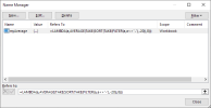
which last can also be defined as a Name using just the first part of the above:

=LAMBDA(a,AVERAGE(TAKE(SORT(TAKE(FILTER(a,a<>"-"),-20)),8)))

and the formula on the sheet becomes:

=myAverage(BG15:BG234)

 

[Peter Bartholomew]

Hi Pascal,
You could make it a lifetime mission to bring all the old solutions up to date! I suspect that reviewing the 'Vault' would throw up some interesting challenges. In the present case, my rework would be simpler, but less robust, than yours.

= AVERAGE(TAKE(SORT(data), 8))

I think the idea of presenting formulas as Lambda functions is a good one in that they expose the intent of the formula without necessarily expecting the user to follow the mechanics. Answers on this forum probably require both the intent and the detail though.