Need the average of the last 4 cells of every 3rd column

[SteveG]

Hi
I've been struggling with this formula for a few days now. Hopefully someone can help. I need a formula that can give me the average of the last 4 of every 3rd cell starting at I.
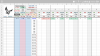
So I need F8 to be the average result of the last 4 entries of every 3rd cell in row 8 with a range between I8:OU8.
For example; if my entries are as follows; I8 =4, L8=12, 08=6, R8= 18, U8=8, the last 4 entries i need to average are 8,18,6,&12 which that divided by 4 would be 44/4 = 10. So F8 would then show 10.

Attached is a photo of the actually spreadsheet I am working on to help clarify. This one is a toughy so I hope someone can help. I would prefer not to use an arrayformula if avoidable but at this point I'll be happy with any solutuon

 

[NARAYANK991]

Hi ,

It might help if you can upload your workbook.

Narayan

 

[SteveG]

How do I do that

 

[bosco_yip]

Try......

Average of the last 4 cells of every 3rd column.

In F8, enter formula :

=AVERAGE(N(OFFSET(G8,0,(MATCH(9^9,8:8)-17)+{1,4,7,10})))

Edit : The result in F8 shall be 11 (44/4), not 10 as stated in Post #.1

Regards
Bosco

 

[SteveG]

You're correct 44/4 is indeed 11. Late night last night. Good catch.

Tried the formula, for ever I could not get it to work. Perhaps I should be more detailed. The average needs to be a running average as I enter new data in. So my range is from i8u8 and I need the last 4 entries of every 3rd column either starting with I8 or starting at ou8 and working nack. I would like it to skip any cells with no data. So basically I need cell i8, L8, O8, R8, U8 and so on to OU8. But I only need the last for of those as they are entered. Perhaps a link to my spreadsheet would help.

https://docs.google.com/spreadsheet...2N6dvrtVQmdE-aH2v9TlaZ18bsQ/edit?usp=drivesdk

As always, any help is great appreciated

 

[bosco_yip]

You're correct 44/4 is indeed 11. Late night last night. Good catch.

Tried the formula, for ever I could not get it to work. Perhaps I should be more detailed. The average needs to be a running average as I enter new data in. So my range is from i8u8 and I need the last 4 entries of every 3rd column either starting with I8 or starting at ou8 and working nack. I would like it to skip any cells with no data. So basically I need cell i8, L8, O8, R8, U8 and so on to OU8. But I only need the last for of those as they are entered. Perhaps a link to my spreadsheet would help.

https://docs.google.com/spreadsheet...2N6dvrtVQmdE-aH2v9TlaZ18bsQ/edit?usp=drivesdk

As always, any help is great appreciated

Average Last 4 of heading "Diff"

1] Please be noted that your attached file is a Google worksheet.

2] I herein attached a Excel file with 2 formula suggestion for your selection :

=AVERAGE(N(OFFSET(G8,0,(MATCH(9^9,G8:OU8)-11)+{1,4,7,10})))

or,

=AVERAGE(N(OFFSET(G8,0,(COUNT(G8:OU8)-11)+{1,4,7,10})))

3] Since Excel function is some different from Google function, if the above formula could not get it to work, try to get help from Google forum.

Regards
Bosco

 

[SteveG]

It's close. Both formulas calculate but it's giving me what the average of the 4 average is instead of averaging the last 4 together. I have it written for both excel and google sheets. Just posted the wrong format. But the formula is calculating, but it's just giving me what the 4th to last average was. So if I have 6,7,8,9 . It's giving me 6. If the next average is 10 it gives me 7. I need it to take the last 4 and average those together. So an average of the averages so to speak. Ie The average of 6+7+8+9 or what ever the last 4 are

 

[bosco_yip]

It's close. Both formulas calculate but it's giving me what the average of the 4 average is instead of averaging the last 4 together. I have it written for both excel and google sheets. Just posted the wrong format. But the formula is calculating, but it's just giving me what the 4th to last average was. So if I have 6,7,8,9 . It's giving me 6. If the next average is 10 it gives me 7. I need it to take the last 4 and average those together. So an average of the averages so to speak. Ie The average of 6+7+8+9 or what ever the last 4 are

1] Please refer to the my post #.6 attached file example of which based on your post #.1 provided information :
I8 =4, L8=12, O8=6, R8= 18, U8=8.
The formula result in F8 show 11.

2] If you have any question, please based of this file.

Regards
Bosco

 

[SteveG]

Thank you for the help. I'll keep looking. I need the formula to add the last 4 and then average it. I8 + L8 + O8 + R8 and then when U8 is add it drops I8 and calculates the average of L8 + O8 + R8 + U8. and when X8 is entered it drops L8 and calculates the average of O8 + R8 + U8+X8 and so on all the way to OU8. Perhaps I asked the question the wrong way. I do appreciate your help though.

In your example F8 should be the average of 12+6+18+8 which is L8 + O8 + R8 + U8 or the last four in that row. F8 Should then = 11 not 12 . F9 in your example would average the sum of -7+10+6+3 F9 should = 3 not -7. F10 would average the sum of 3+8+ -2 + 6. And so on

 

[bosco_yip]

In your example F8 should be the average of 12+6+18+8 which is L8 + O8 + R8 + U8 or the last four in that row. F8 Should then = 11 not 12 . F9 in your example would average the sum of -7+10+6+3 F9 should = 3 not -7. F10 would average the sum of 3+8+ -2 + 6. And so on

This is the screenshot of my posted example.

The formula in F8 show 11 and F9 show 3, that is the correct result.

Are you using Google sheet to open the Excel file ?

Regards

 

[SteveG]

Yep, that's what I was doing wrong. My phone was automatically set to open in google sheets. It works in excel perfectly. Thank you so much. I will still need to figure out how to get it to work in google, since some of the people that will be using it will be on Google. But at least the people that are using excel will have it work correctly. Thank you very much for your help.

 

[SteveG]

Figured it out for google sheets as well

=average(index(G8:8,0,count(G8:8)),index(G8:8,0,(count(G8:8))-3),index(G8:8,0,(count(G8:8))-6),index(G8:8,0,(count(G8:8))-9),index(G8:8,0,(count(G8:8))-12))

 

[Ufoo]

Average Last 4 of heading "Diff"

1] Please be noted that your attached file is a Google worksheet.

2] I herein attached a Excel file with 2 formula suggestion for your selection :

=AVERAGE(N(OFFSET(G8,0,(MATCH(9^9,G8:OU8)-11)+{1,4,7,10})))

or,

=AVERAGE(N(OFFSET(G8,0,(COUNT(G8:OU8)-11)+{1,4,7,10})))

3] Since Excel function is some different from Google function, if the above formula could not get it to work, try to get help from Google forum.

Regards
Bosco

Thanks a lot @bosco_yip for these great formulas. I would kindly request that you unravel the formulas for me/some of us. I thank you in advance for your help.