You are using an out of date browser. It may not display this or other websites correctly.
You should upgrade or use an alternative browser.
You should upgrade or use an alternative browser.
Lookup formula with matching multiple columns
- Thread starter Nandakumar
- Start date

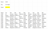
Hi @Nandakumar. Try this array formula (after entering, press Ctrl+Shift+Enter, not just Enter) if you have Excel 365/2021 (or Excel with FILTER/TEXTJOIN support): C7 =TEXTJOIN(", ", TRUE, FILTER(C$11:M$11, INDEX(C12:M22, MATCH(C3, B12:B22, 0), 0) = C5))
Or if you have an old version of Excel (without FILTER, TEXTJOIN). You can use an array formula (after entering, press Ctrl+Shift+Enter, not just Enter): C7 =INDEX(C$11:M$11, MATCH(TRUE, INDEX((INDEX(C12:M22, MATCH(C3, B12:B22, 0), 0)=C5), 0), 0))
These formulas will work for the example file you provided. I hope these formulas will solve your problem. Good luck.
Nandakumar
Member
Hi @MikeVol - it works.Thank you so muchHi @Nandakumar. Try this array formula (after entering, press Ctrl+Shift+Enter, not just Enter) if you have Excel 365/2021 (or Excel with FILTER/TEXTJOIN support): C7 =TEXTJOIN(", ", TRUE, FILTER(C$11:M$11, INDEX(C12:M22, MATCH(C3, B12:B22, 0), 0) = C5))
Or if you have an old version of Excel (without FILTER, TEXTJOIN). You can use an array formula (after entering, press Ctrl+Shift+Enter, not just Enter): C7 =INDEX(C$11:M$11, MATCH(TRUE, INDEX((INDEX(C12:M22, MATCH(C3, B12:B22, 0), 0)=C5), 0), 0))
These formulas will work for the example file you provided. I hope these formulas will solve your problem. Good luck.
AlanSidman
Well-Known Member
Nandakumar
Member
Thank you so muchAn alternative is to create parameter queries in Power Query. See attached. Fill in the parameters and then on the data tab, select Data, RefreshAll
Nandakumar
Member
Hi @MikeVol - I need help on the formula.If i want to change the scenario if name repeats.Attached excel sheet for referenceHi @Nandakumar. Try this array formula (after entering, press Ctrl+Shift+Enter, not just Enter) if you have Excel 365/2021 (or Excel with FILTER/TEXTJOIN support): C7 =TEXTJOIN(", ", TRUE, FILTER(C$11:M$11, INDEX(C12:M22, MATCH(C3, B12:B22, 0), 0) = C5))
Or if you have an old version of Excel (without FILTER, TEXTJOIN). You can use an array formula (after entering, press Ctrl+Shift+Enter, not just Enter): C7 =INDEX(C$11:M$11, MATCH(TRUE, INDEX((INDEX(C12:M22, MATCH(C3, B12:B22, 0), 0)=C5), 0), 0))
These formulas will work for the example file you provided. I hope these formulas will solve your problem. Good luck.
Attachments
p45cal
Well-Known Member
Code:
=TOROW(FILTER(IF(C13:K23=C5,C12:K12,NA()),B13:B23=C3),3)
In the case where the same name visits the same city in the same month more than once you may want to wrap the result in UNIQUE:
Code:
=UNIQUE(TOROW(FILTER(IF(C13:K23=C5,C12:K12,NA()),B13:B23=C3),3),TRUE)
Last edited:
Nandakumar
Member
Hi
,Code:=TOROW(FILTER(IF(C13:K23=C5,C12:K12,NA()),B13:B23=C3),3)
View attachment 90345
In the case where the same name visits the same city in the same month more than once you may want to wrap the result in UNIQUE:
Code:=UNIQUE(TOROW(FILTER(IF(C13:K23=C5,C12:K12,NA()),B13:B23=C3),3),TRUE)
Nandakumar
Member
Hi
Thanks for the formula.
How to extend the formula for the third column and nth column?
Thanks for the formula.
How to extend the formula for the third column and nth column?
p45cal
Well-Known Member
If there are more columns it will show them.Hi
Thanks for the formula.
How to extend the formula for the third column and nth column?

Nandakumar
Member
Hi - I tried formula is not coming for 3rd column.Attached herewith excel sheet for your reference.Please help.
Hi
Attachments
Nandakumar
Member
Thanks got it.There is no Delhi in Sept for A123
I tweaked the data,but answer is coming in ascending based on month instead on actual basis.Attached excel sheet with expected answer.
Attachments
p45cal
Well-Known Member
Take the ,TRUE out that I highlighted with a red oblong in my msg#11, and if you want to see repeating months then take out the UNIQUE wrapper too.I tweaked the data,but answer is coming in ascending based on month instead on actual basis.Attached excel sheet with expected answer.
Nandakumar
Member
p45cal
Well-Known Member
Why?!Hi - how to change the formula to specific cells instead of dynamic arrays.
For example i want to put the formula for D7,E7,F7 instead of automatically taking the formulas to other columns?
Attached excel sheet for your reference
=INDEX(TOROW(FILTER(IF($C$13:$K$23=C5,$C$12:$K$12,NA()),$B$13:$B$23=C3),3),1)
will give you the first result.
=INDEX(TOROW(FILTER(IF($C$13:$K$23=C5,$C$12:$K$12,NA()),$B$13:$B$23=C3),3),2)
will give you the second result etc.
Nandakumar
Member
Thanks you so muchWhy?!
=INDEX(TOROW(FILTER(IF($C$13:$K$23=C5,$C$12:$K$12,NA()),$B$13:$B$23=C3),3),1)
will give you the first result.
=INDEX(TOROW(FILTER(IF($C$13:$K$23=C5,$C$12:$K$12,NA()),$B$13:$B$23=C3),3),2)
will give you the second result etc.
") it works
it works