Pete Wright
Member
Hello! I'm new to this Forum and this is my first question (actually a couple of questions) which I already asked on the Google Groups Discussions a few days ago, but I don't expect an answer there soon, so I am cross-posting my questions here (sorry for that).
So, here we go:
I have the following example table:
There is a group of 3 columns for each month
What I want:
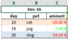
result as on following screenshot:

1) If 2nd cell of a group of 3 columns contains specific text, all three cells should be formatted in a specific color.
Example:
2nd cell = "cat" => background color = red
B3="cat" => A3:C3=<red background>
E4="cat" => D4:F4=<red background>
H3="cat" => G3:I3=<red background>
etc.
2nd cell = "dog" => background color = blue
B5="dog" => A5:C5=<blue background>
E5="dog" => D5:F5=<blue background>
H4="dog" => G4:I4=<blue background>
H5="dog" => G5:I5=<blue background>
etc.
2) The group which shows current month should be formatted in specific color.
Example:
Today is 01/18/2017, so the three merged cells containing "Jan-17" should be formatted. In Addition the three cells below showing the title should be formatted too.
D1=<current month> => D1 (D1:F1)=<yellow background>
D1=<current month> => D2:F2=<yellow background>
Could somebody please explain how to achieve this?
Thanks in advance
Pete
So, here we go:
I have the following example table:
There is a group of 3 columns for each month
Code:
    A     B        C        D    E        F        G    H      I    ...
1        Dec-16         |        Jan-17        |      Feb-17
  ----------------------|----------------------|---------------------
2  day | pet |  amount  | day | pet |  amount  | day | pet |  amount
  ----------------------|----------------------|---------------------
3  10. | cat | -10.00 € | 03. | rat |  12.00 € | 12. | cat | -36.00 €
4  19. | pig |   7.00 € | 07. | cat | -45.00 € | 24. | dog |   8.00 €
5  20. | dog | -34.00 € | 25. | dog | -28.00 € | 24. | dog | -26.00 €
...
What I want:
result as on following screenshot:
1) If 2nd cell of a group of 3 columns contains specific text, all three cells should be formatted in a specific color.
Example:
2nd cell = "cat" => background color = red
B3="cat" => A3:C3=<red background>
E4="cat" => D4:F4=<red background>
H3="cat" => G3:I3=<red background>
etc.
2nd cell = "dog" => background color = blue
B5="dog" => A5:C5=<blue background>
E5="dog" => D5:F5=<blue background>
H4="dog" => G4:I4=<blue background>
H5="dog" => G5:I5=<blue background>
etc.
2) The group which shows current month should be formatted in specific color.
Example:
Today is 01/18/2017, so the three merged cells containing "Jan-17" should be formatted. In Addition the three cells below showing the title should be formatted too.
D1=<current month> => D1 (D1:F1)=<yellow background>
D1=<current month> => D2:F2=<yellow background>
Could somebody please explain how to achieve this?
Thanks in advance
Pete
Attachments
Last edited:
")