DashboardNovice
Member
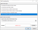
On sheet 1, I have a conditional format formula applied to column D.

The values in column D turn red because the VLOOKUP doesn't recognize these values in column I even though they are there. The reason is because the values in column D are formatted as text instead of number. So far so good.
Because the values in column D are really in column I, and I want the values in column D to be recognized by the VLOOKUP, I need to convert column D to number format.
On sheet 2, I copy the '1' in cell F3, select D7:D26, right click > Paste Special > Multiply. The values in column D are no longer red because they match column I. While this is what I want, I noticed that after multiplying by '1', when I go back and check column D for my conditional format formulas, they are no longer there.
Why did the CF formulas disappear? How can I retain them after multiplying column D by '1?'
