Conditional Format

[Thomas Kuriakose]

Respected Sirs,

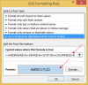
We have a calendar in Sheet1, with units, start date and end date.

In Sheet2, we have mapped the cell reference based on the row and column intersection fr the week numbers.

How can we apply conditional format in Sheet1 to highlight the weeks for the respective unit based on the start date week.

We have colored the cells for the first three units manually

Kindly find attached the file for your reference.

Thank you very much for your help on this.

with regards,
thomas

 

[NARAYANK991]

Hi ,

See the attached file.

Narayan

 

[Thomas Kuriakose]

Respected Sir,

Thank you very much for this solution provided.

Much much appreciated.

Sir, it there a way to do this without the lookup table.

Thank you very much once again,

with regards,
thomas

 

[NARAYANK991]

Hi ,

See the attached file.

Narayan

 

[Thomas Kuriakose]

Respected Sir,

Thank you so much for the second option.

Much much appreciated,

Thanks once again,

with regards,
thomas

 

[Thomas Kuriakose]

Respected Sir,

A new requirement for the conditional format.

We have made the calendar for two years now. In this case, how can we get the week number aligned to the corresponding year to conditional format the correct cell.

Kindly find attached the updated file with years 2018 and 2019 for your reference.

Thank you very much,

with regards,
thomas

 

[bosco_yip]

See attached file.



Regards
Bosco

 

[Thomas Kuriakose]

Respected Sir,

Thank you very much for this solution.

Sir, if we have to use the table reference as in the first solution provided, kindly guide on how to use this.

Thank you very much,

Much appreciated.

with regards,
thomas

 

[bosco_yip]

See revised file with formula revised in

1] Sheet2 B2, copied down :

=WEEKNUM(Sheet1!C4)+(YEAR(Sheet1!C4)=2019)*36

2] Sheet2 D2, copied down :

=B2+4

Regards
Bosco

 

[Thomas Kuriakose]

Respected Sir,

Thank you very much for the revised solution for the table.

Much much appreciated,

with regards,
thomas