Average in Grand Total of Pivot table

[trprasad78]

Hi

I need to help to get Row Average from Row Grand Total.

I have attached Sample file in "Sheet 2" end of Pivotable Column U is expected out put.
It has to come inside the pivot , if use Calculated fields its showing all the columns.

But I need Average after Grand total along with given data on sheet 2.

Please do the needful.
Thank you in advance.

Regards,
Prasad.

 

[vletm]

One quick way ...

 

[trprasad78]

One quick way ...

Thank you , can you explain how you did

 

[trprasad78]

how only sum count allow showing in columns and Grand total showing sum and average

 

[vletm]

Did You even check PivotTable Fields?
Did You notice that there are hidden some columns?
That would be more useful if those Totals could be left side!

 

[trprasad78]

Did You even check PivotTable Fields?
Did You notice that there are hidden some columns?
That would be more useful if those Totals could be left side!

Thank you any chance to remove those column with out hide

 

[vletm]

If You remove those then ... Total Average will remove too.
I would use VBA to solve this.

 

[Debaser]

You can do it by using the data model (assuming you have a version of Excel with it available) and then creating a column set.

 

[trprasad78]

You can do it by using the data model (assuming you have a version of Excel with it available) and then creating a column set.

yes I have latest version , can you share the steps or screen shot where I can do this average

 

[Debaser]

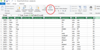
Make the source data into a table, then load it into the data model using the Power Pivot tab:


then create a pivot table:


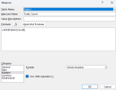
Now create two measures (right click the table name in the pivot table field list, then choose Add measure. The first one is TotalCount:

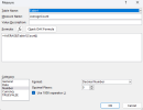
Then AverageCount:




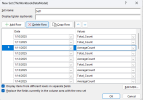
Set up the pivot table as you want it and add both measures to the values area. Now click the Fields, Items and Sets button on the PivotTable Analyze tab and create a column set. You then just delete the columns you don't want to stay in the pivot table - i.e. all the Average ones apart from the total:


That will create a pivot table that only shows the average column at the grand total level.

Note though that this is specific to the dates you have at the time. If you need it to update as you add new dates to the data, you will need to edit the MDX for the set, which is a little more complicated.

 

[trprasad78]

Make the source data into a table, then load it into the data model using the Power Pivot tab:
View attachment 89602

then create a pivot table:
View attachment 89603

Now create two measures (right click the table name in the pivot table field list, then choose Add measure. The first one is TotalCount:
View attachment 89604
Then AverageCount:

View attachment 89605


Set up the pivot table as you want it and add both measures to the values area. Now click the Fields, Items and Sets button on the PivotTable Analyze tab and create a column set. You then just delete the columns you don't want to stay in the pivot table - i.e. all the Average ones apart from the total:
View attachment 89606

That will create a pivot table that only shows the average column at the grand total level.

Note though that this is specific to the dates you have at the time. If you need it to update as you add new dates to the data, you will need to edit the MDX for the set, which is a little more complicated.

thank you so much for your time and explanation , let me check and get back