copied formula skipping rows

[APAY]

Hi!
Really need help today if possible. I've tried copying other suggested formulas from other formulas but just cant get this to work for me.

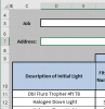
I have data in cells in Sheet 1 that need to be copied to Sheet 2. I have 2 issues to overcome.
(1) The cell to be copied to in Sheet 2 is a merge of 3 rows. Referring to my sample data attached: If I say in Sheet 2 B3 that it equals Sheet 1 C2 when I copy this down to B6 it pulls C5 from Sheet 1 instead of C3.

(2) I want Sheet 2 C2 to equal Sheet 1 A2. The I want it to skip row C3 and copy that formula down to C4. ie. it skips every 2nd row but pulls the sequenced data from the first sheet.

I have seen the MOD function used but cant get my head around how to apply the division to my worksheet. I'm really not an expert in these formulas so please be detailed with suggestions ie. if I need to reference a sheet inside brackets tell me which one. lol

Thanks for you help.

 

[NARAYANK991]

Hi ,

See the attached file.

Narayan

 

[APAY]

Hi ,

See the attached file.

Narayan

Thanks for your Reply,

In your formula below for Sheet 2 C2, how do I adapt the Mod row bit for my actual spreadsheet (not the one sent to you) where the field I'm picking is a merged field of 3 columns starting at row 11. ie. Sheet1 C11:E11?
=IF(MOD((ROW()-1),3)=0,

At the moment if I use your formula with the changed sheet names and cell references it just shows up blank.

The set up is the same as I displayed in the sample for Sheet 2 but my cell reference is D3 where in my sample it was Sheet 2 C2 (if that effects the MOD Row function)

PS. I've attached a screen shot of how I tried to do the formula if that helps

 

[NARAYANK991]

Hi ,

I am sorry but I am not able to understand the problem.

In your uploaded sample workbook , you had Sheet1 and Sheet2 , where Sheet1 had the input data in tabular form and Sheet2 displayed it in the format you wanted.

In your uploaded sample workbook Sheet1 did not have any merged cells.

In the screenshot which you have attached with your latest post , the sheet name Lighting List is used ; is this your input data sheet ?

Even when you use merged cells in a formula , you should use only the top left hand corner cell reference , the reference that is shown in the Name Box when you place the cursor in the merged cells. Thus , your formula should use 'Lighting List'!C11 instead of 'Lighting List'!C11:E11.

Narayan

 

[APAY]

Yes 'Lighting List' is my real Sheet 1 equivalent. I cant upload the real spreadsheet I'm working on as I need to protect data.

The screen shot I just upload is from my actual Lighting List sheet so in cell D3 of Sheet2 (see my last screen shot) I put this formula.

=IF(MOD((ROW()-1),3)=0,"",OFFSET('Lighting List'!C11,INT((ROW() - ROW('Lighting List'!C11))/3), MOD((ROW() - ROW('Lighting List'!C11)),3)))

I think the mod row bit needs to be adjusted to reflect the cell references in my actual spreadsheet but I dont know what to change it to.

Hope that makes sense.

 

[NARAYANK991]

Hi ,

Can you see if this works ?

=IF(MOD((ROW()-2),3)=0,"",OFFSET('Lighting List'!C11,INT((ROW() - ROW(D$3))/3), MOD((ROW() - ROW(D$3)),3)))

The highlighted references are to the first cell where this formula is entered.

The part (ROW()-2) was earlier (ROW()-1) ; the change means that cells D3 and D4 will have outputs in them , and D5 will be blank. Is this what you want ?

Narayan

 

[APAY]

Almost. This put the right reference in D3 then skipped D4 & D5 (which I want it to do) then in D6 which should equal Lighting List C12 it selects Lighting List C14.

To make it easier I have created another sample excel sheet with the fields in the same locations as my spreadsheet.

Also, how do you work out the parts of the Row to put in 'MOD((ROW()-2),3)=0,'? I will need to apply this formula to other columns of the sheet and need to know what to do to adapt it.

Thanks for your help!

 

[NARAYANK991]

Hi ,

See the attached file.

I will explain the formula in another post.

Narayan

 

[APAY]

Thanks for that. Looking forward to the explanation as I cant figure out how to apply what you have done to other columns in that top row.

 

[NARAYANK991]

Hi ,

To explain the formula , let us consider the following one :

=IF(MOD((ROW()-2),3)=0,"",OFFSET('Lighting List'!C$11,INT((ROW() - ROW(D$3))/3), 6 * MOD((ROW() - ROW(D$3)),3)))

The first part , which is :

=IF(MOD((ROW()-2),3)=0,"",

will decide which row or rows will be blank ; in this case , since the check is for the MOD value being zero , only one row , the third one in each block of 3 cells , will be blank.

In case this is difficult to visualize , just step through the rows , starting from row #3 which is the first row.

Row 3 ...... ROW() - 2 = 1 ...... MOD(1,3) = 1 <> 0 , will be populated

Row 4 ...... ROW() - 2 = 2 ...... MOD(2,3) = 2 <> 0 , will be populated

Row 5 ...... ROW() - 2 = 3 ...... MOD(3,3) = 0 = 0 , will be blank

Row 6 ...... ROW() - 2 = 4 ...... MOD(4,3) = 1 <> 0 , will be populated

Row 7 ...... ROW() - 2 = 5 ...... MOD(5,3) = 2 <> 0 , will be populated

Row 8 ...... ROW() - 2 = 6 ...... MOD(6,3) = 0 = 0 , will be blank

If you want more than one row to be blank , and if your grouping is 3 rows forming a block , then the following :

=IF(MOD((ROW()-3),3) <> 0,"",

will ensure that the first row is populated with data , and the remaining two rows in each block will be blank.

Suppose you have a block consisting of 4 cells , and you want that the first two cells in each block should be populated with data while the remaining 2 cells in each block are blank , then the formula would be :

=IF(MOD((ROW()-3),4) > 1,"",

If we work through this as before , we will have :

Row 3 ...... ROW() - 3 = 0 ...... MOD(0,4) = 0 < 2 , will be populated

Row 4 ...... ROW() - 3 = 1 ...... MOD(1,4) = 1 < 2 , will be populated

Row 5 ...... ROW() - 3 = 2 ...... MOD(2,4) = 2 , not < 2 , will be blank

Row 6 ...... ROW() - 3 = 3 ...... MOD(3,4) = 3 , not < 2 , will be blank

Row 7 ...... ROW() - 3 = 4 ...... MOD(4,4) = 0 < 2 , will be populated

Row 8 ...... ROW() - 3 = 5 ...... MOD(5,4) = 1 < 2 , will be populated

Row 9 ...... ROW() - 3 = 6 ...... MOD(6,4) = 2 , not < 2 , will be blank

Row 10 .... ROW() - 3 = 7 ...... MOD(7,4) = 3 , not < 2 , will be blank

I will continue in the next post.

Narayan

 

[APAY]

Thank you for that. This makes it a bit clearer. In the sample you sent back with the formulas I cant understand how Sheet 2 D3 & D4 have the same formula but are pulling the different values from Lighting List sheet.

Also, I tried copying the formula from D3 to G3 and changed the reference in the formula to reference G3 but it still picks up the same data that D3 does from Lighting List Sheet. I have another 15 columns across row 3 in my real spreadsheet that I will need to do the same for but that references different columns in Lighting List Sheet.

 

[NARAYANK991]

Hi ,

If we consider the working part of the formula , which is :

OFFSET('Lighting List'!C$11,INT((ROW() - ROW(D$3))/3), 6 * MOD((ROW() - ROW(D$3)),3))

we have blocks of 3 cells such as D3:D5 , D6:D8 , D9:D11 , D12:D14.

In each block , we need to populate the first 2 cells , while the 3rd will remain blank. The blank cell will be handled by the IF function ; we have discussed this in my earlier post.

The two cells which are to be populated ,need to take their values from C11 and I11.

If we agree that the OFFSET function is the route we should take , then what we want is :

Row 1 ..... D3 ..... OFFSET('Lighting List'!C$11 , 0 , 0)

Row 2 ..... D4 ..... OFFSET('Lighting List'!C$11 , 0 , 6)

Row 4 ..... D6 ..... OFFSET('Lighting List'!C$11 , 1 , 0)

Row 5 ..... D7 ..... OFFSET('Lighting List'!C$11 , 1 , 6)

Row 7 ..... D9 ..... OFFSET('Lighting List'!C$11 , 2 , 0)

Row 8 ..... D10 ... OFFSET('Lighting List'!C$11 , 2 , 6)

Row 10 ... D12 ... OFFSET('Lighting List'!C$11 , 3 , 0)

Row 11 ... D13 ... OFFSET('Lighting List'!C$11 , 3 , 6)

Once we reduce our requirements in this fashion , we can see that the ROW OFFSET needs an INT , while the COLUMN OFFSET needs a MOD.

If you want to know the reason for this , INT will increase as the row number increases , while MOD always toggles within a set number of values depending on the second parameter of the MOD function.

To get the ROW OFFSET , we can use :

INT((ROW(D3) - ROW(D$3)) / 3)

This will give us the following result :

Row 1 ..... D3 ..... 0

Row 2 ..... D4 ..... 0

Row 4 ..... D6 ..... 1

Row 5 ..... D7 ..... 1

Row 7 ..... D9 ..... 2

Row 8 ..... D10 ... 2

Row 10 ... D12 ... 3

Row 11 ... D13 ... 3

To get the COLUMN OFFSET , we can use :

6 * MOD((ROW(D3) - ROW(D$3)) , 3)

This will give us the following result :

Row 1 ..... D3 ..... 0

Row 2 ..... D4 ..... 6

Row 4 ..... D6 ..... 0

Row 5 ..... D7 ..... 6

Row 7 ..... D9 ..... 0

Row 8 ..... D10 ... 6

Row 10 ... D12 ... 0

Row 11 ... D13 ... 6

What ever be your requirement , first reduce it to an OFFSET function with the appropriate ROW OFFSET and COLUMN OFFSET values ; then see how these correlate with the row and / or column numbers where the formula will be entered , and only after that see which expression using INT / MOD will give the desired result.

Narayan