Conditional Formatting - Calendar

[Luis Silva]

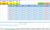
Hello, I´m making a holiday planner for different workers. In monthly worksheet I insert all the different occurrences (pex: x-present, h-holiday, etc), and I use conditional format to highlight the cells with different colors. What I need is a yearly calendar view for each different worker, with dropdown/data validation to choose the worker and after a year calendar that replicates the conditional format used on the monthly worksheet for that worker. Can someone give a help on how to do this, the formula to use in the conditional format, or point out a file that I can see. Thanks

 

[Chihiro]

Here's link to thread for one such calendar.
https://chandoo.org/forum/threads/attendance-calendar-help.30988/#post-184422

Other than that, your question is too generic for us to give pointers.

 

[Luis Silva]

Hi again, thanks for your feedback. I´ve seen your file, it´s very close but i still didn´t make it. Could you please take a look to my file structure. Thanks

 

[Chihiro]

I wouldn't recommend your approach.

Data entry (tracking) should be done in flat table structure. Which makes subsequent reporting/analysis easy.

Don't have time to look at it today. I'll see if I have time tomorrow.

 

[Peter Bartholomew]

I think it is possible by first consolidating the selected individual's record for the year on a hidden sheet. From there the individual's status is can be looked up by day and month using a Named formula based upon the date in the cell. You cannot insert the value on the worksheet without creating a circular reference but you can use it for conditional formatting.

 

[Luis Silva]

Hi Peter, thank you very much for your help! You made it! I thought it was much easier. Visually I like it, but it is very tricky... Like Chihiro, do you recommend another approach for a similar result?

 

[Peter Bartholomew]

Hi Luis, as Chihiro suggests your monthly data input forms are not the most convenient data structure to achieve flexible data reporting. That said, your calendar report does not require much in the way of flexibility and can be built to reference the cross-tab table on the 'hidden' sheet.

The main problem, as I see it, is that the conditional formatting is far more complicated than anything you are used to. For me, it is simpler to use a named formula 'status' because I use named formulas every time I use Excel. You could, alternatively, just type the whole formula into each of the conditional formats using the Rules Manager instead of using 'status' but that is not much better.

My only other solution is that you replicate your year view, either as a new sheet or to one side on the existing sheet. The new cells could be used to look up the "A"s and "P"s from the hidden sheet to correspond to the dates in the Year View. The conditional formats would be build by reference to the new cells.

Or, of course, you could just persevere. Finish your calendar and copy the conditional formats using format painter.

 

[bosco_yip]

1] Set up a calendar planner with formulas

2] Sheet Name to be named in : month+year, e.g. Jan2018, Feb2018…...etc

3] Dropdown list for Month and Year as in C4 and D4

4] Select C6:I11 >> Conditional Formatting >> New rule :

- Rule 1 >> formula :

=ISNUMBER(MATCH(C6,INDEX(AGGREGATE(15,6,COLUMN($A$1:$AE$1)/(INDEX(INDIRECT("'"&$C$4&$D$4&"'!$C$4:$AG$100"),MATCH($B$4,INDIRECT("'"&$C$4&$D$4&"'!$B$4:$B$100"),0),0)="P"),COLUMN($A$1:$AE$1)),0),0))

>> Format cell ground color : Green

- Rule 2 >> formula :

=ISNUMBER(MATCH(C6,INDEX(AGGREGATE(15,6,COLUMN($A$1:$AE$1)/(INDEX(INDIRECT("'"&$C$4&$D$4&"'!$C$4:$AG$100"),MATCH($B$4,INDIRECT("'"&$C$4&$D$4&"'!$B$4:$B$100"),0),0)="A"),COLUMN($A$1:$AE$1)),0),0))

>> Format cell ground color : Pink

Regards
Bosco

 

[Luis Silva]

Hello Bosco,

Thank you very much for your inputs! Excellent, month / year / worker option! But I´m getting an error for some months when updating the calendar (pex: Feb). I still didn´t find where...

 

[bosco_yip]

Hello Bosco,

Thank you very much for your inputs! Excellent, month / year / worker option! But I´m getting an error for some months when updating the calendar (pex: Feb). I still didn´t find where...

Uploaded your file for checking

Regards
Bosco

 

[Luis Silva]

It´s the same I didn´t touch it. I´m using excel 2016.

 

[bosco_yip]

It´s the same I didn´t touch it. I´m using excel 2016.

Hi,

1] The file is OK, I made a little revised in B2 to suit with the sheet name.

2] The file worksheets have Jan2018, Feb2018….... Jan2019 and Feb2019.

Then, for the month of Jan and Feb, your can select 2018 or 2019 and you will find the difference.

Regards
Bosco

 

[Luis Silva]

I´m still getting the error, on months feb, abr, may aug, set out dec

 

[Luis Silva]

The error comes from the calendar itself. If you are not seeing it what can it be?

 

[bosco_yip]

The error comes from the calendar itself. If you are not seeing it what can it be?

Hi,

1] My file is OK, please see the screenshot in post #8

2 ] Maybe the regional Date setting problem

3] My computer used British type Date system, your system maybe in USA type.

4] In the calendar planner, I try to change all formula in USA date system (but I can't checking)

5] Please see revised file

Regards
Bosco

 

[Luis Silva]

Hi Bosco, no that doesn´t work either. Super strange, cause it works for some of the months. I tried to use a month/year calendar model that I already have on the file and it works ok, now I have to adjust the conditional format formulas. If you find the solution please post it. If I cannot make the adjustments to the conditional formulas I will be back in touch with you.
Thanks again for all the help!
Regards,
Luis

 

[Peter Bartholomew]

Hi Bosco, no that (doesn´t) work either.

@Bosco Just to confirm that version 1b works fine on an English UK machine with Office 2010. Not that I have any idea how you manage to write such complex formulas in the conditional formatting dialogue box! Either it requires genius or there is a trick of developing the formula piecemeal before loading it and pulling up the ladder.

Even 'simplifying' through the use of names did not
= ISNUMBER( MATCH( target, INDEX( AGGREGATE( 15, 6, day.array / (INDEX(attendance_forMonth, employee_rowNum, 0)="P"), day.array), 0 ), 0 ) )
where the monthly tables are addressed by locally-scoped names
=INDIRECT("'"&Month&Year&"'!attendance_byMonth")
and the employee row number is given by
=MATCH( Employee, INDIRECT("'"&Month&Year&"'!employee_byMonth"), 0 )

I use the word 'simplifying'; it helps me but, probably, not others

 

[Luis Silva]

Hi again, sorry guys, I confirm also that it works fine changing to British Format at Windows Control Panel (I didn´t change it correctly at the first time). Will try to adapt formula to my date format. Thanks again!

 

[Luis Silva]

Hi Bosco,, I was not able to detect where to change it to my date format (Portuguese format). Could you please give me directions, and if not asking to much explain by words the conditional format formula. Thanks!

 

[bosco_yip]

Hi Bosco,, I was not able to detect where to change it to my date format (Portuguese format). Could you please give me directions, and if not asking to much explain by words the conditional format formula. Thanks!

Are you asking for this one ?



Regards

 

[Luis Silva]

Hi Bosco,

No...

What i really need is the attached file working with your conditional format on my computer (Portuguese Date Format that comes from "Windows Control Panel).

That date location you pointed out on your last post was what I changed the first time, when I said the file still didn´t work on my side.

Regards,
Luis

 

[bosco_yip]

Hi Bosco,

No...

What i really need is the attached file working with your conditional format on my computer (Portuguese Date Format that comes from "Windows Control Panel).

That date location you pointed out on your last post was what I changed the first time, when I said the file still didn´t work on my side.

Regards,
Luis

Hi,

Here's the file fixed in respect of formula revised under the Conditional Formatting.

Regards
Bosco

 

[Luis Silva]

Thank you for all the support!!!
Best Regards,
Luis

 

[Peter Bartholomew]

@Luis Silva
I realise that you are sorted but I wasn't happy with the file as it stood. I modified the formulas to read the input data at source. Each month sheet has a named range using the abbreviation for the month and the function CHOOSE is used to select the correct input data for each calendar month.